Code
pacman::p_load(olsrr, corrplot, ggpubr, sf, spdep, GWmodel, tmap, tidyverse, gtsummary)Muhamad Ameer Noor
December 6, 2023
December 14, 2023

Geographically Weighted Regression (GWR) is a statistical method that considers factors that vary from place to place (like climate, demographics, or physical environment) and models how these factors relate to a specific outcome (dependent variable). This hands-on session will teach you how to create hedonic pricing models using GWR. The focus is on resale prices of condominiums in 2015, with independent variables categorized as structural and locational.
Two datasets will be used:
Before diving in, it’s crucial to install the required R packages and activate them in the R environment.
olsrr: A package designed for tools that assist in the model building and exploratory analysis associated with ordinary least squares regression.
corrplot: A graphical display of a correlation matrix, confidence interval, or general matrix-like visualization to assist with interpretative analysis.
ggpubr: An ‘ggplot2’ extension that simplifies creating beautiful graphics for publication, offering an easy-to-use set of tools for descriptive statistics and a rich array of plots.
sf: This package provides simple and straightforward ways to handle and manipulate spatial vector data in R, integrating tightly with the ‘tidyverse’ and ‘ggplot2’.
spdep: Spatial dependence: weighting schemes, statistics, and models; a collection of functions to create spatial weights matrix objects from polygon contiguities, from point patterns by distance and tessellations, for summarizing these objects, and for permitting their use in spatial data models.
GWmodel: An R package for fitting Geographically Weighted Models, which are spatial statistical models that allow local rather than global parameters to be estimated.
tmap: An R library for creating thematic maps, which are designed to represent spatial variation of a subject using statistical data.
tidyverse: An opinionated collection of R packages designed for data science tasks that make it easy to import, tidy, transform, and visualize data.
gtsummary: This package provides an elegant and flexible way to create publication-ready analytical and summary tables using the ‘gt’ package, integrating with ‘broom’ and ‘tidyverse’ workflows.
The GWmodel package offers a set of localized spatial statistical methods. These include GW summary statistics, GW principal components analysis, GW discriminant analysis, and various forms of GW regression, some of which are robust (resistant to outliers). Typically, the results or parameters from GWmodel are visually mapped, serving as an insightful exploration tool. This often comes before or guides more traditional or advanced statistical analyses.
In this practical exercise, we’ll be using geospatial data named MP14_SUBZONE_WEB_PL. It’s in ESRI shapefile format and represents URA Master Plan 2014’s planning subzone boundaries. These geographic boundaries are depicted using polygon features, and the GIS data uses the svy21 projected coordinate system.
The code snippet below demonstrates how to import the MP14_SUBZONE_WEB_PL shapefile using the st_read() function from the sf package.
Reading layer `MP14_SUBZONE_WEB_PL' from data source
  `C:\ameernoor\ISSS624\data\geospatial' using driver `ESRI Shapefile'
Simple feature collection with 323 features and 15 fields
Geometry type: MULTIPOLYGON
Dimension:     XY
Bounding box:  xmin: 2667.538 ymin: 15748.72 xmax: 56396.44 ymax: 50256.33
Projected CRS: SVY21
The report above indicates that the R object containing the imported shapefile is named mpsz, and it’s a simple feature object with a geometry type of multipolygon. It’s important to note that the mpsz object lacks EPSG information.
The following code snippet ensures that the recently imported mpsz is updated with the correct ESPG code, which is 3414.
Once the projection metadata is transformed, you can check the projection of the updated mpsz_svy21 using st_crs() from the sf package.
The code below will be used to check the updated mpsz_svy21.
Coordinate Reference System:
  User input: EPSG:3414
  wkt:
PROJCRS["SVY21 / Singapore TM",
    BASEGEOGCRS["SVY21",
        DATUM["SVY21",
            ELLIPSOID["WGS 84",6378137,298.257223563,
                LENGTHUNIT["metre",1]]],
        PRIMEM["Greenwich",0,
            ANGLEUNIT["degree",0.0174532925199433]],
        ID["EPSG",4757]],
    CONVERSION["Singapore Transverse Mercator",
        METHOD["Transverse Mercator",
            ID["EPSG",9807]],
        PARAMETER["Latitude of natural origin",1.36666666666667,
            ANGLEUNIT["degree",0.0174532925199433],
            ID["EPSG",8801]],
        PARAMETER["Longitude of natural origin",103.833333333333,
            ANGLEUNIT["degree",0.0174532925199433],
            ID["EPSG",8802]],
        PARAMETER["Scale factor at natural origin",1,
            SCALEUNIT["unity",1],
            ID["EPSG",8805]],
        PARAMETER["False easting",28001.642,
            LENGTHUNIT["metre",1],
            ID["EPSG",8806]],
        PARAMETER["False northing",38744.572,
            LENGTHUNIT["metre",1],
            ID["EPSG",8807]]],
    CS[Cartesian,2],
        AXIS["northing (N)",north,
            ORDER[1],
            LENGTHUNIT["metre",1]],
        AXIS["easting (E)",east,
            ORDER[2],
            LENGTHUNIT["metre",1]],
    USAGE[
        SCOPE["Cadastre, engineering survey, topographic mapping."],
        AREA["Singapore - onshore and offshore."],
        BBOX[1.13,103.59,1.47,104.07]],
    ID["EPSG",3414]]
Now, you’ll see that the EPSG code is listed as 3414.
Next, to see the full extent of mpsz_svy21, you can use st_bbox() from the sf package.
mpsz is transformed to CRS 3414.mpsz_svy21.mpsz_svy21.The condo_resale_2015 data comes in CSV format. The code below uses the read_csv() function from the readr package to bring condo_resale_2015 into R, and it becomes a tibble data frame named condo_resale.
After importing the data, it’s essential to check if everything is in order. The code snippets below, using glimpse(), help you understand the structure of the data.
Rows: 1,436
Columns: 23
$ LATITUDE             <dbl> 1.287145, 1.328698, 1.313727, 1.308563, 1.321437,…
$ LONGITUDE            <dbl> 103.7802, 103.8123, 103.7971, 103.8247, 103.9505,…
$ POSTCODE             <dbl> 118635, 288420, 267833, 258380, 467169, 466472, 3…
$ SELLING_PRICE        <dbl> 3000000, 3880000, 3325000, 4250000, 1400000, 1320…
$ AREA_SQM             <dbl> 309, 290, 248, 127, 145, 139, 218, 141, 165, 168,…
$ AGE                  <dbl> 30, 32, 33, 7, 28, 22, 24, 24, 27, 31, 17, 22, 6,…
$ PROX_CBD             <dbl> 7.941259, 6.609797, 6.898000, 4.038861, 11.783402…
$ PROX_CHILDCARE       <dbl> 0.16597932, 0.28027246, 0.42922669, 0.39473543, 0…
$ PROX_ELDERLYCARE     <dbl> 2.5198118, 1.9333338, 0.5021395, 1.9910316, 1.121…
$ PROX_URA_GROWTH_AREA <dbl> 6.618741, 7.505109, 6.463887, 4.906512, 6.410632,…
$ PROX_HAWKER_MARKET   <dbl> 1.76542207, 0.54507614, 0.37789301, 1.68259969, 0…
$ PROX_KINDERGARTEN    <dbl> 0.05835552, 0.61592412, 0.14120309, 0.38200076, 0…
$ PROX_MRT             <dbl> 0.5607188, 0.6584461, 0.3053433, 0.6910183, 0.528…
$ PROX_PARK            <dbl> 1.1710446, 0.1992269, 0.2779886, 0.9832843, 0.116…
$ PROX_PRIMARY_SCH     <dbl> 1.6340256, 0.9747834, 1.4715016, 1.4546324, 0.709…
$ PROX_TOP_PRIMARY_SCH <dbl> 3.3273195, 0.9747834, 1.4715016, 2.3006394, 0.709…
$ PROX_SHOPPING_MALL   <dbl> 2.2102717, 2.9374279, 1.2256850, 0.3525671, 1.307…
$ PROX_SUPERMARKET     <dbl> 0.9103958, 0.5900617, 0.4135583, 0.4162219, 0.581…
$ PROX_BUS_STOP        <dbl> 0.10336166, 0.28673408, 0.28504777, 0.29872340, 0…
$ NO_Of_UNITS          <dbl> 18, 20, 27, 30, 30, 31, 32, 32, 32, 32, 34, 34, 3…
$ FAMILY_FRIENDLY      <dbl> 0, 0, 0, 0, 0, 1, 1, 0, 1, 1, 0, 0, 0, 0, 0, 0, 0…
$ FREEHOLD             <dbl> 1, 1, 1, 1, 1, 1, 1, 1, 1, 0, 1, 1, 1, 1, 1, 1, 1…
$ LEASEHOLD_99YR <dbl> 0, 0, 0, 0, 0, 0, 0, 0, 0, 0, 0, 0, 0, 0, 0, 0, 0…[1] 103.7802 103.8123 103.7971 103.8247 103.9505 103.9386[1] 1.287145 1.328698 1.313727 1.308563 1.321437 1.314198Next, using the base R function summary(), you can get summary statistics for the cond_resale tibble data frame.
    LATITUDE       LONGITUDE        POSTCODE      SELLING_PRICE
 Min.   :1.240   Min.   :103.7   Min.   : 18965   Min.   :  540000
 1st Qu.:1.309   1st Qu.:103.8   1st Qu.:259849   1st Qu.: 1100000
 Median :1.328   Median :103.8   Median :469298   Median : 1383222
 Mean   :1.334   Mean   :103.8   Mean   :440439   Mean   : 1751211
 3rd Qu.:1.357   3rd Qu.:103.9   3rd Qu.:589486   3rd Qu.: 1950000
 Max.   :1.454   Max.   :104.0   Max.   :828833   Max.   :18000000
    AREA_SQM          AGE           PROX_CBD       PROX_CHILDCARE
 Min.   : 34.0   Min.   : 0.00   Min.   : 0.3869   Min.   :0.004927
 1st Qu.:103.0   1st Qu.: 5.00   1st Qu.: 5.5574   1st Qu.:0.174481
 Median :121.0   Median :11.00   Median : 9.3567   Median :0.258135
 Mean   :136.5   Mean   :12.14   Mean   : 9.3254   Mean   :0.326313
 3rd Qu.:156.0   3rd Qu.:18.00   3rd Qu.:12.6661   3rd Qu.:0.368293
 Max.   :619.0   Max.   :37.00   Max.   :19.1804   Max.   :3.465726
 PROX_ELDERLYCARE  PROX_URA_GROWTH_AREA PROX_HAWKER_MARKET PROX_KINDERGARTEN
 Min.   :0.05451   Min.   :0.2145       Min.   :0.05182    Min.   :0.004927
 1st Qu.:0.61254   1st Qu.:3.1643       1st Qu.:0.55245    1st Qu.:0.276345
 Median :0.94179   Median :4.6186       Median :0.90842    Median :0.413385
 Mean   :1.05351   Mean   :4.5981       Mean   :1.27987    Mean   :0.458903
 3rd Qu.:1.35122   3rd Qu.:5.7550       3rd Qu.:1.68578    3rd Qu.:0.578474
 Max.   :3.94916   Max.   :9.1554       Max.   :5.37435    Max.   :2.229045
    PROX_MRT         PROX_PARK       PROX_PRIMARY_SCH  PROX_TOP_PRIMARY_SCH
 Min.   :0.05278   Min.   :0.02906   Min.   :0.07711   Min.   :0.07711
 1st Qu.:0.34646   1st Qu.:0.26211   1st Qu.:0.44024   1st Qu.:1.34451
 Median :0.57430   Median :0.39926   Median :0.63505   Median :1.88213
 Mean   :0.67316   Mean   :0.49802   Mean   :0.75471   Mean   :2.27347
 3rd Qu.:0.84844   3rd Qu.:0.65592   3rd Qu.:0.95104   3rd Qu.:2.90954
 Max.   :3.48037   Max.   :2.16105   Max.   :3.92899   Max.   :6.74819
 PROX_SHOPPING_MALL PROX_SUPERMARKET PROX_BUS_STOP       NO_Of_UNITS
 Min.   :0.0000     Min.   :0.0000   Min.   :0.001595   Min.   :  18.0
 1st Qu.:0.5258     1st Qu.:0.3695   1st Qu.:0.098356   1st Qu.: 188.8
 Median :0.9357     Median :0.5687   Median :0.151710   Median : 360.0
 Mean   :1.0455     Mean   :0.6141   Mean   :0.193974   Mean   : 409.2
 3rd Qu.:1.3994     3rd Qu.:0.7862   3rd Qu.:0.220466   3rd Qu.: 590.0
 Max.   :3.4774     Max.   :2.2441   Max.   :2.476639   Max.   :1703.0
 FAMILY_FRIENDLY     FREEHOLD      LEASEHOLD_99YR
 Min.   :0.0000   Min.   :0.0000   Min.   :0.0000
 1st Qu.:0.0000   1st Qu.:0.0000   1st Qu.:0.0000
 Median :0.0000   Median :0.0000   Median :0.0000
 Mean   :0.4868   Mean   :0.4227   Mean   :0.4882
 3rd Qu.:1.0000   3rd Qu.:1.0000   3rd Qu.:1.0000
Max. :1.0000 Max. :1.0000 Max. :1.0000 Currently, condo_resale is a tibble data frame without spatial information. Let’s convert it into a sf object. The code below transforms condo_resale into a simple feature data frame using st_as_sf() from the sf package.
Note that st_transform() from the sf package is used to change the coordinates from wgs84 (i.e., crs:4326) to svy21 (i.e., crs=3414).
Next, using head(), you can check the content of condo_resale.sf.
Simple feature collection with 6 features and 21 fields
Geometry type: POINT
Dimension:     XY
Bounding box:  xmin: 22085.12 ymin: 29951.54 xmax: 41042.56 ymax: 34546.2
Projected CRS: SVY21 / Singapore TM
# A tibble: 6 × 22
  POSTCODE SELLING_PRICE AREA_SQM   AGE PROX_CBD PROX_CHILDCARE PROX_ELDERLYCARE
     <dbl>         <dbl>    <dbl> <dbl>    <dbl>          <dbl>            <dbl>
1   118635       3000000      309    30     7.94          0.166            2.52
2   288420       3880000      290    32     6.61          0.280            1.93
3   267833       3325000      248    33     6.90          0.429            0.502
4   258380       4250000      127     7     4.04          0.395            1.99
5   467169       1400000      145    28    11.8           0.119            1.12
6   466472       1320000      139    22    10.3           0.125            0.789
# ℹ 15 more variables: PROX_URA_GROWTH_AREA <dbl>, PROX_HAWKER_MARKET <dbl>,
#   PROX_KINDERGARTEN <dbl>, PROX_MRT <dbl>, PROX_PARK <dbl>,
#   PROX_PRIMARY_SCH <dbl>, PROX_TOP_PRIMARY_SCH <dbl>,
#   PROX_SHOPPING_MALL <dbl>, PROX_SUPERMARKET <dbl>, PROX_BUS_STOP <dbl>,
#   NO_Of_UNITS <dbl>, FAMILY_FRIENDLY <dbl>, FREEHOLD <dbl>,
#   LEASEHOLD_99YR <dbl>, geometry <POINT [m]>
The output now represents a point feature data frame.
In this part, you’ll discover how to use visual tools from the ggplot2 package for Exploratory Data Analysis (EDA).
To understand the distribution of SELLING_PRICE, check out the code below. It generates a histogram:
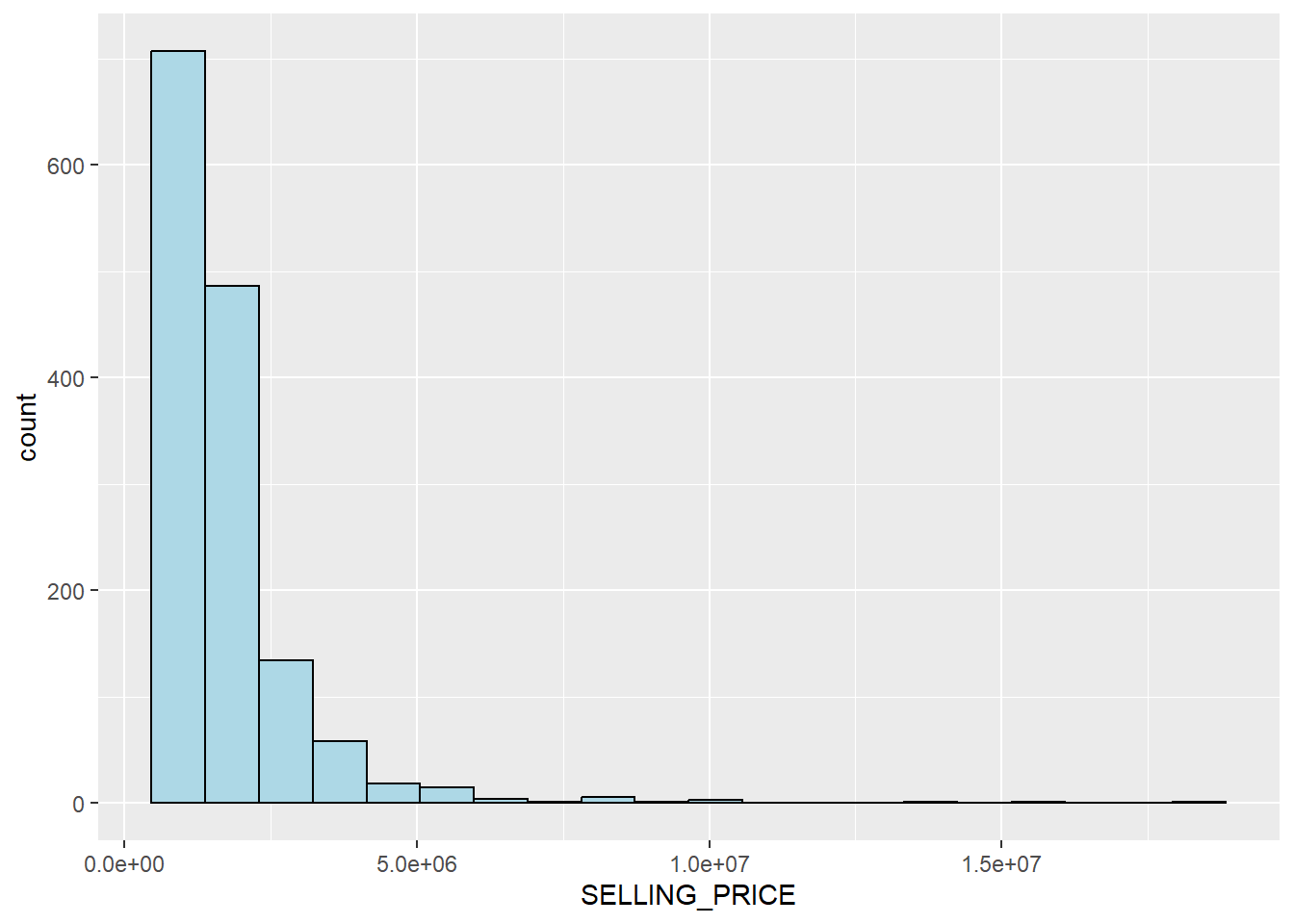
The graph above shows a right-skewed distribution, indicating more condos were sold at relatively lower prices.
Statistically, we can normalize the skewed distribution by applying a log transformation. The following code creates a new variable, LOG_SELLING_PRICE, using the log transformation on SELLING_PRICE with mutate() from the dplyr package.
Now, you can plot LOG_SELLING_PRICE using the code below.
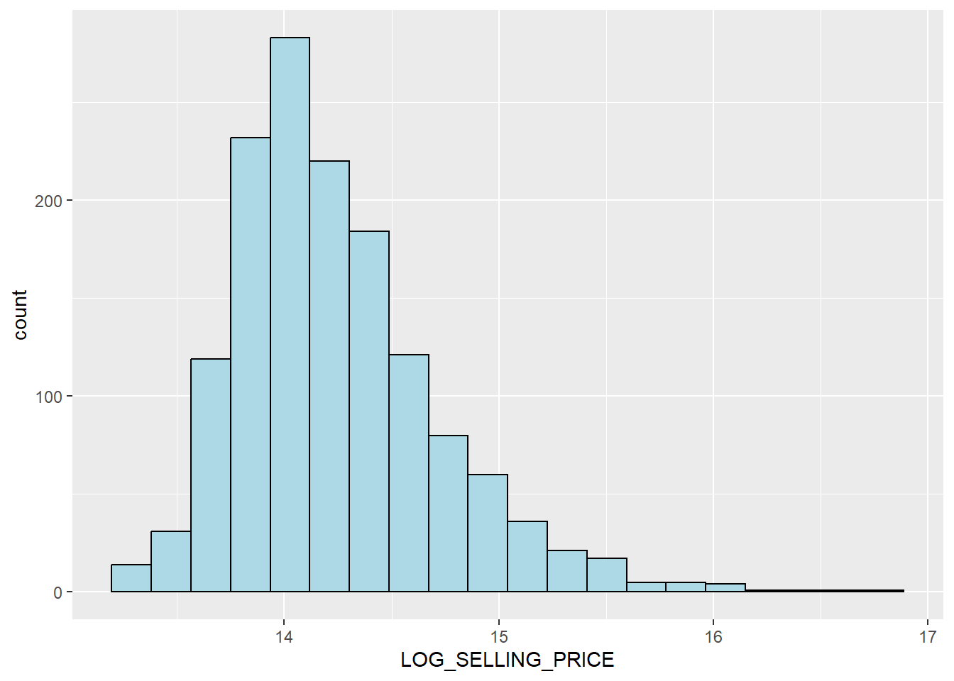
Notice that the distribution is less skewed after the transformation.
In this part, you’ll learn to create a set of small multiple histograms (also called trellis plots) using ggarrange() from the ggpubr package.
The code below generates 12 histograms and organizes them into a 3-column by 4-row layout using ggarrange().
AREA_SQM <- ggplot(data=condo_resale.sf, aes(x= `AREA_SQM`)) +
  geom_histogram(bins=20, color="black", fill="light blue")

AGE <- ggplot(data=condo_resale.sf, aes(x= `AGE`)) +
  geom_histogram(bins=20, color="black", fill="light blue")

PROX_CBD <- ggplot(data=condo_resale.sf, aes(x= `PROX_CBD`)) +
  geom_histogram(bins=20, color="black", fill="light blue")

PROX_CHILDCARE <- ggplot(data=condo_resale.sf, aes(x= `PROX_CHILDCARE`)) +
  geom_histogram(bins=20, color="black", fill="light blue")

PROX_ELDERLYCARE <- ggplot(data=condo_resale.sf, aes(x= `PROX_ELDERLYCARE`)) +
  geom_histogram(bins=20, color="black", fill="light blue")

PROX_URA_GROWTH_AREA <- ggplot(data=condo_resale.sf,
                               aes(x= `PROX_URA_GROWTH_AREA`)) +
  geom_histogram(bins=20, color="black", fill="light blue")

PROX_HAWKER_MARKET <- ggplot(data=condo_resale.sf, aes(x= `PROX_HAWKER_MARKET`)) +
  geom_histogram(bins=20, color="black", fill="light blue")

PROX_KINDERGARTEN <- ggplot(data=condo_resale.sf, aes(x= `PROX_KINDERGARTEN`)) +
  geom_histogram(bins=20, color="black", fill="light blue")

PROX_MRT <- ggplot(data=condo_resale.sf, aes(x= `PROX_MRT`)) +
  geom_histogram(bins=20, color="black", fill="light blue")

PROX_PARK <- ggplot(data=condo_resale.sf, aes(x= `PROX_PARK`)) +
  geom_histogram(bins=20, color="black", fill="light blue")

PROX_PRIMARY_SCH <- ggplot(data=condo_resale.sf, aes(x= `PROX_PRIMARY_SCH`)) +
  geom_histogram(bins=20, color="black", fill="light blue")

PROX_TOP_PRIMARY_SCH <- ggplot(data=condo_resale.sf,
                               aes(x= `PROX_TOP_PRIMARY_SCH`)) +
  geom_histogram(bins=20, color="black", fill="light blue")

ggarrange(AREA_SQM, AGE, PROX_CBD, PROX_CHILDCARE, PROX_ELDERLYCARE,
          PROX_URA_GROWTH_AREA, PROX_HAWKER_MARKET, PROX_KINDERGARTEN, PROX_MRT,
          PROX_PARK, PROX_PRIMARY_SCH, PROX_TOP_PRIMARY_SCH,
          ncol = 3, nrow = 4)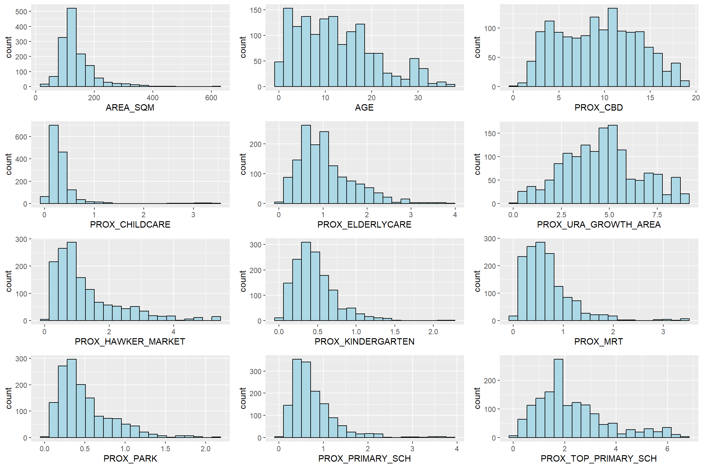
Finally, let’s visualize the geographic distribution of condominium resale prices in Singapore. We’ll use the tmap package for this.
# activate interactive mode
tmap_mode("plot")

# correct the invalid geometry
fixed_geom <- sf::st_make_valid(mpsz_svy21[mpsz_svy21$REGION_N == "CENTRAL REGION", ])

# create the map
tm_shape(fixed_geom)+
  tm_polygons() +
tm_shape(condo_resale.sf) +
  tm_dots(col = "SELLING_PRICE",
          alpha = 0.6,
          style="quantile") +
  tm_view(set.zoom.limits = c(11,14))
Note that we’re using tm_dots() instead of tm_bubbles().
The set.zoom.limits parameter in tm_view() sets the minimum and maximum zoom level to 11 and 14, respectively.
Before moving on to the next section, switch R display back to plot mode using the code below:
In this part, you’ll understand how to create hedonic pricing models for resale condominiums using the lm() function in the R base.
First, we’ll make a simple linear regression model. We’ll use SELLING_PRICE as the result we want to predict and AREA_SQM as the factor we think influences it.
The lm() function gives us a result object, and we can get more details using functions like summary():
Call:
lm(formula = SELLING_PRICE ~ AREA_SQM, data = condo_resale.sf)

Residuals:
     Min       1Q   Median       3Q      Max
-3695815  -391764   -87517   258900 13503875

Coefficients:
             Estimate Std. Error t value Pr(>|t|)
(Intercept) -258121.1    63517.2  -4.064 5.09e-05 ***
AREA_SQM      14719.0      428.1  34.381  < 2e-16 ***
---
Signif. codes:  0 '***' 0.001 '**' 0.01 '*' 0.05 '.' 0.1 ' ' 1

Residual standard error: 942700 on 1434 degrees of freedom
Multiple R-squared:  0.4518,    Adjusted R-squared:  0.4515
F-statistic:  1182 on 1 and 1434 DF,  p-value: < 2.2e-16
The report shows that the SELLING_PRICE can be estimated using the formula:
*y = -258121.1 + 14719x1*An R-squared value of 0.4518 indicates that our model explains about 45% of resale prices.
With a p-value much smaller than 0.0001, we reject the idea that the average is a good estimate of SELLING_PRICE. This lets us conclude that our simple linear regression model is a good estimator.
In the Coefficients: section, both Intercept and AREA_SQM have p-values smaller than 0.001, suggesting we reject the null hypothesis for B0 and B1. Thus, we can infer that B0 and B1 are good parameter estimates.
To visualize the best-fit line on a scatterplot, we can use lm() as a method function in ggplot’s geometry:
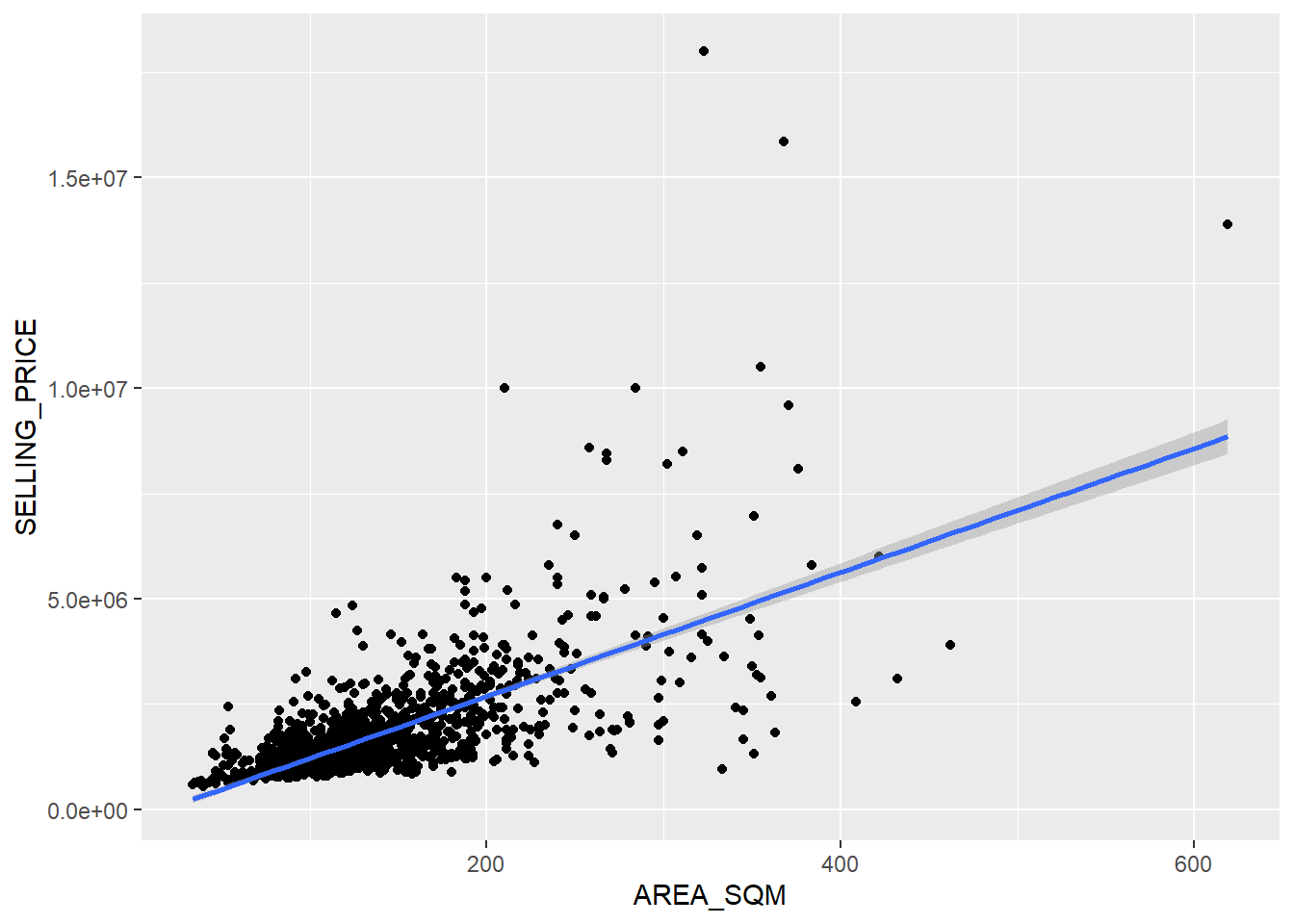
This figure reveals some statistical outliers with relatively high selling prices.
Before creating a multiple regression model, it’s crucial to check that independent variables aren’t highly correlated. If they are, it can compromise the model quality, a phenomenon known as multicollinearity in statistics.
A correlation matrix is commonly used to visualize relationships between independent variables. The corrplot package can help with this. The code below generates a scatterplot matrix for the independent variables in the condo_resale data.frame.
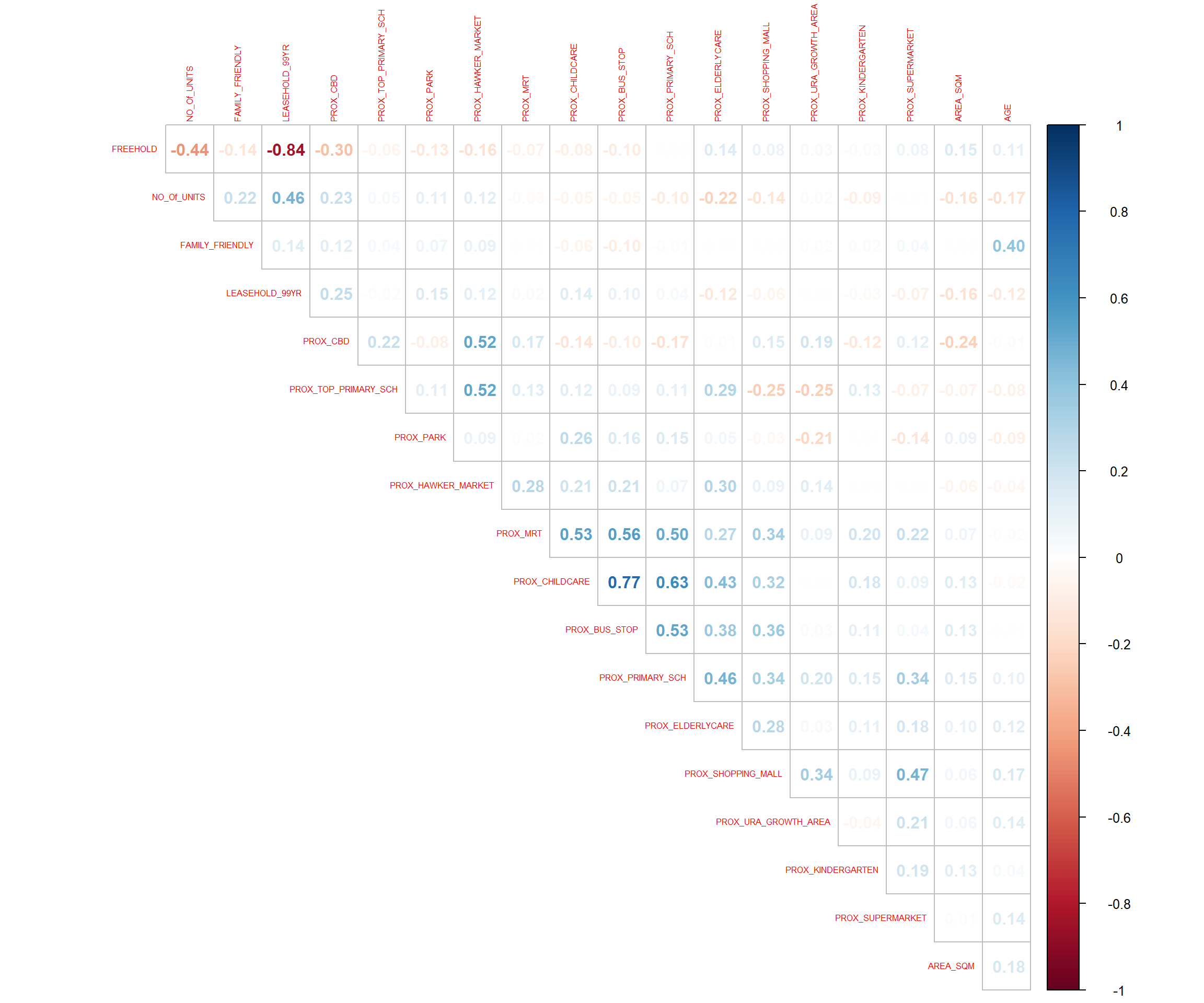
Matrix reorder is crucial for mining hidden structures and patterns. Four methods in corrplot (parameter order) are available: “AOE”, “FPC”, “hclust”, “alphabet”. In the above code, AOE order is used, ordering variables using the angular order of the eigenvectors method suggested by Michael Friendly.
The scatterplot matrix reveals that Freehold is highly correlated with LEASE_99YEAR. To avoid multicollinearity, it’s wise to include only one of them in the subsequent model. As a result, LEASE_99YEAR is excluded in the next model.
The code below uses lm() to build the multiple linear regression model.
condo.mlr <- lm(formula = SELLING_PRICE ~ AREA_SQM + AGE +
                  PROX_CBD + PROX_CHILDCARE + PROX_ELDERLYCARE +
                  PROX_URA_GROWTH_AREA + PROX_HAWKER_MARKET + PROX_KINDERGARTEN +
                  PROX_MRT  + PROX_PARK + PROX_PRIMARY_SCH +
                  PROX_TOP_PRIMARY_SCH + PROX_SHOPPING_MALL + PROX_SUPERMARKET +
                  PROX_BUS_STOP + NO_Of_UNITS + FAMILY_FRIENDLY + FREEHOLD,
                data=condo_resale.sf)
summary(condo.mlr)
Call:
lm(formula = SELLING_PRICE ~ AREA_SQM + AGE + PROX_CBD + PROX_CHILDCARE +
    PROX_ELDERLYCARE + PROX_URA_GROWTH_AREA + PROX_HAWKER_MARKET +
    PROX_KINDERGARTEN + PROX_MRT + PROX_PARK + PROX_PRIMARY_SCH +
    PROX_TOP_PRIMARY_SCH + PROX_SHOPPING_MALL + PROX_SUPERMARKET +
    PROX_BUS_STOP + NO_Of_UNITS + FAMILY_FRIENDLY + FREEHOLD,
    data = condo_resale.sf)

Residuals:
     Min       1Q   Median       3Q      Max
-3475964  -293923   -23069   241043 12260381

Coefficients:
                       Estimate Std. Error t value Pr(>|t|)
(Intercept)           481728.40  121441.01   3.967 7.65e-05 ***
AREA_SQM               12708.32     369.59  34.385  < 2e-16 ***
AGE                   -24440.82    2763.16  -8.845  < 2e-16 ***
PROX_CBD              -78669.78    6768.97 -11.622  < 2e-16 ***
PROX_CHILDCARE       -351617.91  109467.25  -3.212  0.00135 **
PROX_ELDERLYCARE      171029.42   42110.51   4.061 5.14e-05 ***
PROX_URA_GROWTH_AREA   38474.53   12523.57   3.072  0.00217 **
PROX_HAWKER_MARKET     23746.10   29299.76   0.810  0.41782
PROX_KINDERGARTEN     147468.99   82668.87   1.784  0.07466 .
PROX_MRT             -314599.68   57947.44  -5.429 6.66e-08 ***
PROX_PARK             563280.50   66551.68   8.464  < 2e-16 ***
PROX_PRIMARY_SCH      180186.08   65237.95   2.762  0.00582 **
PROX_TOP_PRIMARY_SCH    2280.04   20410.43   0.112  0.91107
PROX_SHOPPING_MALL   -206604.06   42840.60  -4.823 1.57e-06 ***
PROX_SUPERMARKET      -44991.80   77082.64  -0.584  0.55953
PROX_BUS_STOP         683121.35  138353.28   4.938 8.85e-07 ***
NO_Of_UNITS             -231.18      89.03  -2.597  0.00951 **
FAMILY_FRIENDLY       140340.77   47020.55   2.985  0.00289 **
FREEHOLD              359913.01   49220.22   7.312 4.38e-13 ***
---
Signif. codes:  0 '***' 0.001 '**' 0.01 '*' 0.05 '.' 0.1 ' ' 1

Residual standard error: 755800 on 1417 degrees of freedom
Multiple R-squared:  0.6518,    Adjusted R-squared:  0.6474
F-statistic: 147.4 on 18 and 1417 DF, p-value: < 2.2e-16From the report, not all independent variables are statistically significant. We’ll refine the model by removing those variables that aren’t statistically significant. The code below recalibrates the model.
                             Model Summary
------------------------------------------------------------------------
R                       0.807       RMSE                     755957.289
R-Squared               0.651       Coef. Var                    43.168
Adj. R-Squared          0.647       MSE                571471422208.591
Pred R-Squared          0.638       MAE                      414819.628
------------------------------------------------------------------------
 RMSE: Root Mean Square Error
 MSE: Mean Square Error
 MAE: Mean Absolute Error

                                     ANOVA
--------------------------------------------------------------------------------
                    Sum of
                   Squares          DF         Mean Square       F         Sig.
--------------------------------------------------------------------------------
Regression    1.512586e+15          14        1.080418e+14    189.059    0.0000
Residual      8.120609e+14        1421    571471422208.591
Total         2.324647e+15        1435
--------------------------------------------------------------------------------

                                               Parameter Estimates
-----------------------------------------------------------------------------------------------------------------
               model           Beta    Std. Error    Std. Beta       t        Sig           lower          upper
-----------------------------------------------------------------------------------------------------------------
         (Intercept)     527633.222    108183.223                   4.877    0.000     315417.244     739849.200
            AREA_SQM      12777.523       367.479        0.584     34.771    0.000      12056.663      13498.382
                 AGE     -24687.739      2754.845       -0.167     -8.962    0.000     -30091.739     -19283.740
            PROX_CBD     -77131.323      5763.125       -0.263    -13.384    0.000     -88436.469     -65826.176
      PROX_CHILDCARE    -318472.751    107959.512       -0.084     -2.950    0.003    -530249.889    -106695.613
    PROX_ELDERLYCARE     185575.623     39901.864        0.090      4.651    0.000     107302.737     263848.510
PROX_URA_GROWTH_AREA      39163.254     11754.829        0.060      3.332    0.001      16104.571      62221.936
            PROX_MRT    -294745.107     56916.367       -0.112     -5.179    0.000    -406394.234    -183095.980
           PROX_PARK     570504.807     65507.029        0.150      8.709    0.000     442003.938     699005.677
    PROX_PRIMARY_SCH     159856.136     60234.599        0.062      2.654    0.008      41697.849     278014.424
  PROX_SHOPPING_MALL    -220947.251     36561.832       -0.115     -6.043    0.000    -292668.213    -149226.288
       PROX_BUS_STOP     682482.221    134513.243        0.134      5.074    0.000     418616.359     946348.082
         NO_Of_UNITS       -245.480        87.947       -0.053     -2.791    0.005       -418.000        -72.961
     FAMILY_FRIENDLY     146307.576     46893.021        0.057      3.120    0.002      54320.593     238294.560
            FREEHOLD     350599.812     48506.485        0.136      7.228    0.000     255447.802     445751.821
-----------------------------------------------------------------------------------------------------------------The gtsummary package offers an elegant way to create publication-ready summary tables in R.
In the code below, tbl_regression() creates a well-formatted regression report.
| Characteristic | Beta | 95% CI1 | p-value |
|---|---|---|---|
| (Intercept) | 527,633 | 315,417, 739,849 | <0.001 |
| AREA_SQM | 12,778 | 12,057, 13,498 | <0.001 |
| AGE | -24,688 | -30,092, -19,284 | <0.001 |
| PROX_CBD | -77,131 | -88,436, -65,826 | <0.001 |
| PROX_CHILDCARE | -318,473 | -530,250, -106,696 | 0.003 |
| PROX_ELDERLYCARE | 185,576 | 107,303, 263,849 | <0.001 |
| PROX_URA_GROWTH_AREA | 39,163 | 16,105, 62,222 | <0.001 |
| PROX_MRT | -294,745 | -406,394, -183,096 | <0.001 |
| PROX_PARK | 570,505 | 442,004, 699,006 | <0.001 |
| PROX_PRIMARY_SCH | 159,856 | 41,698, 278,014 | 0.008 |
| PROX_SHOPPING_MALL | -220,947 | -292,668, -149,226 | <0.001 |
| PROX_BUS_STOP | 682,482 | 418,616, 946,348 | <0.001 |
| NO_Of_UNITS | -245 | -418, -73 | 0.005 |
| FAMILY_FRIENDLY | 146,308 | 54,321, 238,295 | 0.002 |
| FREEHOLD | 350,600 | 255,448, 445,752 | <0.001 |
| 1 CI = Confidence Interval | |||
With gtsummary, model statistics can be included using add_glance_table() or as a table source note using add_glance_source_note(), as shown below.
| Characteristic | Beta | 95% CI1 | p-value |
|---|---|---|---|
| (Intercept) | 527,633 | 315,417, 739,849 | <0.001 |
| AREA_SQM | 12,778 | 12,057, 13,498 | <0.001 |
| AGE | -24,688 | -30,092, -19,284 | <0.001 |
| PROX_CBD | -77,131 | -88,436, -65,826 | <0.001 |
| PROX_CHILDCARE | -318,473 | -530,250, -106,696 | 0.003 |
| PROX_ELDERLYCARE | 185,576 | 107,303, 263,849 | <0.001 |
| PROX_URA_GROWTH_AREA | 39,163 | 16,105, 62,222 | <0.001 |
| PROX_MRT | -294,745 | -406,394, -183,096 | <0.001 |
| PROX_PARK | 570,505 | 442,004, 699,006 | <0.001 |
| PROX_PRIMARY_SCH | 159,856 | 41,698, 278,014 | 0.008 |
| PROX_SHOPPING_MALL | -220,947 | -292,668, -149,226 | <0.001 |
| PROX_BUS_STOP | 682,482 | 418,616, 946,348 | <0.001 |
| NO_Of_UNITS | -245 | -418, -73 | 0.005 |
| FAMILY_FRIENDLY | 146,308 | 54,321, 238,295 | 0.002 |
| FREEHOLD | 350,600 | 255,448, 445,752 | <0.001 |
| R² = 0.651; Adjusted R² = 0.647; AIC = 42,967; Statistic = 189; p-value = <0.001; σ = 755,957 | |||
| 1 CI = Confidence Interval | |||
For more customization options, refer to Tutorial: tbl_regression
In this section, we’ll introduce a powerful R package designed for OLS regression - olsrr. It offers valuable methods for enhancing multiple linear regression models:
The code chunk below uses the ols_vif_tol() function of the olsrr package to test for signs of multicollinearity.
              Variables Tolerance      VIF
1              AREA_SQM 0.8728554 1.145665
2                   AGE 0.7071275 1.414172
3              PROX_CBD 0.6356147 1.573280
4        PROX_CHILDCARE 0.3066019 3.261559
5      PROX_ELDERLYCARE 0.6598479 1.515501
6  PROX_URA_GROWTH_AREA 0.7510311 1.331503
7              PROX_MRT 0.5236090 1.909822
8             PROX_PARK 0.8279261 1.207837
9      PROX_PRIMARY_SCH 0.4524628 2.210126
10   PROX_SHOPPING_MALL 0.6738795 1.483945
11        PROX_BUS_STOP 0.3514118 2.845664
12          NO_Of_UNITS 0.6901036 1.449058
13      FAMILY_FRIENDLY 0.7244157 1.380423
14             FREEHOLD 0.6931163 1.442759
Since the VIF of the independent variables is less than 10, we can conclude that there are no signs of multicollinearity among the independent variables.
It’s essential to test the assumption of linearity and additivity of the relationship between dependent and independent variables in multiple linear regression.
In the code chunk below, the ols_plot_resid_fit() function of the olsrr package is used to perform a linearity assumption test.
The figure above reveals that most data points scatter around the 0 line, suggesting that the relationships between the dependent variable and independent variables are linear.
Finally, the code chunk below uses ols_plot_resid_hist() of the olsrr package to perform a normality assumption test.
The figure indicates that the residual of the multiple linear regression model (i.e., condo.mlr1) resembles a normal distribution.
If you prefer formal statistical tests, the ols_test_normality() of the olsrr package can be used, as shown in the code chunk below.
-----------------------------------------------
       Test             Statistic       pvalue
-----------------------------------------------
Shapiro-Wilk              0.6856         0.0000
Kolmogorov-Smirnov        0.1366         0.0000
Cramer-von Mises         121.0768        0.0000
Anderson-Darling         67.9551         0.0000
-----------------------------------------------
The summary table above shows that the p-values of the four tests are much smaller than the alpha value of 0.05. Therefore, we reject the null hypothesis, indicating there is statistical evidence that the residuals are not normally distributed.
Since our hedonic model uses geographically referenced attributes, visualizing the residuals is crucial.
To perform a spatial autocorrelation test, we’ll convert condo_resale.sf from an sf data frame into a SpatialPointsDataFrame.
First, export the residuals of the hedonic pricing model and save them as a data frame.
Next, join the newly created data frame with condo_resale.sf.
Now, convert condo_resale.res.sf from a simple feature object into a SpatialPointsDataFrame since the spdep package processes sp-conformed spatial data objects.
The code chunk below performs the data conversion process.
class       : SpatialPointsDataFrame
features    : 1436
extent      : 14940.85, 43352.45, 24765.67, 48382.81  (xmin, xmax, ymin, ymax)
crs         : +proj=tmerc +lat_0=1.36666666666667 +lon_0=103.833333333333 +k=1 +x_0=28001.642 +y_0=38744.572 +ellps=WGS84 +towgs84=0,0,0,0,0,0,0 +units=m +no_defs
variables   : 23
names       : POSTCODE, SELLING_PRICE, AREA_SQM, AGE,    PROX_CBD, PROX_CHILDCARE, PROX_ELDERLYCARE, PROX_URA_GROWTH_AREA, PROX_HAWKER_MARKET, PROX_KINDERGARTEN,    PROX_MRT,   PROX_PARK, PROX_PRIMARY_SCH, PROX_TOP_PRIMARY_SCH, PROX_SHOPPING_MALL, ...
min values  :    18965,        540000,       34,   0, 0.386916393,    0.004927023,      0.054508623,          0.214539508,        0.051817113,       0.004927023, 0.052779424, 0.029064164,      0.077106132,          0.077106132,                  0, ...
max values  :   828833,       1.8e+07,      619,  37, 19.18042832,     3.46572633,      3.949157205,           9.15540001,        5.374348075,       2.229045366,  3.48037319,  2.16104919,      3.928989144,          6.748192062,        3.477433767, ...
Next, use the tmap package to display the distribution of residuals on an interactive map.
The code churn below turns on the interactive mode of tmap.
The code chunks below create an interactive point symbol map.
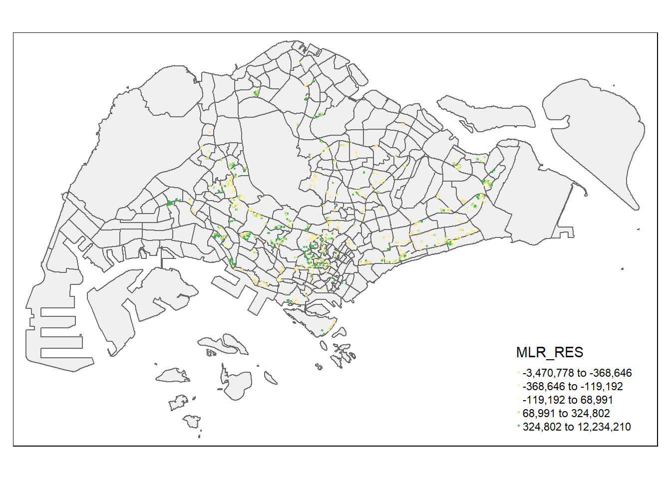
Remember to switch back to “plot” mode before continuing.
The figure above reveals signs of spatial autocorrelation.
To verify our observation, the Moran’s I test will be performed.
First, compute the distance-based weight matrix using dnearneigh() function of the spdep package.
Neighbour list object:
Number of regions: 1436
Number of nonzero links: 66266
Percentage nonzero weights: 3.213526
Average number of links: 46.14624
10 disjoint connected subgraphs
Link number distribution:

  1   3   5   7   9  10  11  12  13  14  15  16  17  18  19  20  21  22  23  24
  3   3   9   4   3  15  10  19  17  45  19   5  14  29  19   6  35  45  18  47
 25  26  27  28  29  30  31  32  33  34  35  36  37  38  39  40  41  42  43  44
 16  43  22  26  21  11   9  23  22  13  16  25  21  37  16  18   8  21   4  12
 45  46  47  48  49  50  51  52  53  54  55  56  57  58  59  60  61  62  63  64
  8  36  18  14  14  43  11  12   8  13  12  13   4   5   6  12  11  20  29  33
 65  66  67  68  69  70  71  72  73  74  75  76  77  78  79  80  81  82  83  84
 15  20  10  14  15  15  11  16  12  10   8  19  12  14   9   8   4  13  11   6
 85  86  87  88  89  90  91  92  93  94  95  96  97  98  99 100 101 102 103 104
  4   9   4   4   4   6   2  16   9   4   5   9   3   9   4   2   1   2   1   1
105 106 107 108 109 110 112 116 125
  1   5   9   2   1   3   1   1   1
3 least connected regions:
193 194 277 with 1 link
1 most connected region:
285 with 125 links
Next, use nb2listw() of the spdep package to convert the output neighbors lists (i.e., nb) into spatial weights.
Characteristics of weights list object:
Neighbour list object:
Number of regions: 1436
Number of nonzero links: 66266
Percentage nonzero weights: 3.213526
Average number of links: 46.14624
10 disjoint connected subgraphs
Link number distribution:

  1   3   5   7   9  10  11  12  13  14  15  16  17  18  19  20  21  22  23  24
  3   3   9   4   3  15  10  19  17  45  19   5  14  29  19   6  35  45  18  47
 25  26  27  28  29  30  31  32  33  34  35  36  37  38  39  40  41  42  43  44
 16  43  22  26  21  11   9  23  22  13  16  25  21  37  16  18   8  21   4  12
 45  46  47  48  49  50  51  52  53  54  55  56  57  58  59  60  61  62  63  64
  8  36  18  14  14  43  11  12   8  13  12  13   4   5   6  12  11  20  29  33
 65  66  67  68  69  70  71  72  73  74  75  76  77  78  79  80  81  82  83  84
 15  20  10  14  15  15  11  16  12  10   8  19  12  14   9   8   4  13  11   6
 85  86  87  88  89  90  91  92  93  94  95  96  97  98  99 100 101 102 103 104
  4   9   4   4   4   6   2  16   9   4   5   9   3   9   4   2   1   2   1   1
105 106 107 108 109 110 112 116 125
  1   5   9   2   1   3   1   1   1
3 least connected regions:
193 194 277 with 1 link
1 most connected region:
285 with 125 links

Weights style: W
Weights constants summary:
     n      nn   S0       S1       S2
W 1436 2062096 1436 94.81916 5798.341
Now, use lm.morantest() of the spdep package to perform Moran’s I test for residual spatial autocor
relation.
    Global Moran I for regression residuals

data:
model: lm(formula = SELLING_PRICE ~ AREA_SQM + AGE + PROX_CBD +
PROX_CHILDCARE + PROX_ELDERLYCARE + PROX_URA_GROWTH_AREA + PROX_MRT +
PROX_PARK + PROX_PRIMARY_SCH + PROX_SHOPPING_MALL + PROX_BUS_STOP +
NO_Of_UNITS + FAMILY_FRIENDLY + FREEHOLD, data = condo_resale.sf)
weights: nb_lw

Moran I statistic standard deviate = 24.366, p-value < 2.2e-16
alternative hypothesis: greater
sample estimates:
Observed Moran I      Expectation         Variance
    1.438876e-01    -5.487594e-03     3.758259e-05
The Global Moran’s I test for residual spatial autocorrelation shows that its p-value is less than 0.00000000000000022, which is less than the alpha value of 0.05. Hence, we reject the null hypothesis that the residuals are randomly distributed.
Since the Observed Global Moran I = 0.1424418, which is greater than 0, we can infer that the residuals resemble a cluster distribution.
In this section, you’ll learn how to model hedonic pricing using both fixed and adaptive bandwidth schemes.
In the code chunk below, the bw.gwr() function of the GWModel package is used to determine the optimal fixed bandwidth for the model. The argument adaptive set to FALSE indicates that we want to compute the fixed bandwidth.
There are two possible approaches to determine the stopping rule: CV cross-validation and AIC corrected (AICc). The stopping rule is defined using the approach argument.
bw.fixed <- bw.gwr(formula = SELLING_PRICE ~ AREA_SQM + AGE + PROX_CBD +
                     PROX_CHILDCARE + PROX_ELDERLYCARE  + PROX_URA_GROWTH_AREA +
                     PROX_MRT   + PROX_PARK + PROX_PRIMARY_SCH +
                     PROX_SHOPPING_MALL + PROX_BUS_STOP + NO_Of_UNITS +
                     FAMILY_FRIENDLY + FREEHOLD,
                   data=condo_resale.sp,
                   approach="CV",
                   kernel="gaussian",
                   adaptive=FALSE,
                   longlat=FALSE)
Fixed bandwidth: 17660.96 CV score: 8.259118e+14
Fixed bandwidth: 10917.26 CV score: 7.970454e+14
Fixed bandwidth: 6749.419 CV score: 7.273273e+14
Fixed bandwidth: 4173.553 CV score: 6.300006e+14
Fixed bandwidth: 2581.58 CV score: 5.404958e+14
Fixed bandwidth: 1597.687 CV score: 4.857515e+14
Fixed bandwidth: 989.6077 CV score: 4.722431e+14
Fixed bandwidth: 613.7939 CV score: 1.378294e+16
Fixed bandwidth: 1221.873 CV score: 4.778717e+14
Fixed bandwidth: 846.0596 CV score: 4.791629e+14
Fixed bandwidth: 1078.325 CV score: 4.751406e+14
Fixed bandwidth: 934.7772 CV score: 4.72518e+14
Fixed bandwidth: 1023.495 CV score: 4.730305e+14
Fixed bandwidth: 968.6643 CV score: 4.721317e+14
Fixed bandwidth: 955.7206 CV score: 4.722072e+14
Fixed bandwidth: 976.6639 CV score: 4.721387e+14
Fixed bandwidth: 963.7202 CV score: 4.721484e+14
Fixed bandwidth: 971.7199 CV score: 4.721293e+14
Fixed bandwidth: 973.6083 CV score: 4.721309e+14
Fixed bandwidth: 970.5527 CV score: 4.721295e+14
Fixed bandwidth: 972.4412 CV score: 4.721296e+14
Fixed bandwidth: 971.2741 CV score: 4.721292e+14
Fixed bandwidth: 970.9985 CV score: 4.721293e+14
Fixed bandwidth: 971.4443 CV score: 4.721292e+14
Fixed bandwidth: 971.5496 CV score: 4.721293e+14
Fixed bandwidth: 971.3793 CV score: 4.721292e+14
Fixed bandwidth: 971.3391 CV score: 4.721292e+14
Fixed bandwidth: 971.3143 CV score: 4.721292e+14
Fixed bandwidth: 971.3545 CV score: 4.721292e+14
Fixed bandwidth: 971.3296 CV score: 4.721292e+14
Fixed bandwidth: 971.345 CV score: 4.721292e+14
Fixed bandwidth: 971.3355 CV score: 4.721292e+14
Fixed bandwidth: 971.3413 CV score: 4.721292e+14
Fixed bandwidth: 971.3377 CV score: 4.721292e+14
Fixed bandwidth: 971.34 CV score: 4.721292e+14
Fixed bandwidth: 971.3405 CV score: 4.721292e+14
Fixed bandwidth: 971.3408 CV score: 4.721292e+14
Fixed bandwidth: 971.3403 CV score: 4.721292e+14
Fixed bandwidth: 971.3406 CV score: 4.721292e+14
Fixed bandwidth: 971.3404 CV score: 4.721292e+14
Fixed bandwidth: 971.3405 CV score: 4.721292e+14
Fixed bandwidth: 971.3405 CV score: 4.721292e+14 The result shows that the recommended bandwidth is 971.3405 meters. (Quiz: Do you know why it is in meters?)
Now we can calibrate the gwr model using the fixed bandwidth and a Gaussian kernel, as shown in the code chunk below.
gwr.fixed <- gwr.basic(formula = SELLING_PRICE ~ AREA_SQM + AGE + PROX_CBD +
                         PROX_CHILDCARE + PROX_ELDERLYCARE  + PROX_URA_GROWTH_AREA +
                         PROX_MRT   + PROX_PARK + PROX_PRIMARY_SCH +
                         PROX_SHOPPING_MALL + PROX_BUS_STOP + NO_Of_UNITS +
                         FAMILY_FRIENDLY + FREEHOLD,
                       data=condo_resale.sp,
                       bw=bw.fixed,
                       kernel = 'gaussian',
                       longlat = FALSE)
The output is saved in a list of class “gwrm”. The code below can be used to display the model output.
   ***********************************************************************
   *                       Package   GWmodel                             *
   ***********************************************************************
   Program starts at: 2023-12-18 02:18:04.568794
   Call:
   gwr.basic(formula = SELLING_PRICE ~ AREA_SQM + AGE + PROX_CBD +
    PROX_CHILDCARE + PROX_ELDERLYCARE + PROX_URA_GROWTH_AREA +
    PROX_MRT + PROX_PARK + PROX_PRIMARY_SCH + PROX_SHOPPING_MALL +
    PROX_BUS_STOP + NO_Of_UNITS + FAMILY_FRIENDLY + FREEHOLD,
    data = condo_resale.sp, bw = bw.fixed, kernel = "gaussian",
    longlat = FALSE)

   Dependent (y) variable:  SELLING_PRICE
   Independent variables:  AREA_SQM AGE PROX_CBD PROX_CHILDCARE PROX_ELDERLYCARE PROX_URA_GROWTH_AREA PROX_MRT PROX_PARK PROX_PRIMARY_SCH PROX_SHOPPING_MALL PROX_BUS_STOP NO_Of_UNITS FAMILY_FRIENDLY FREEHOLD
   Number of data points: 1436
   ***********************************************************************
   *                    Results of Global Regression                     *
   ***********************************************************************

   Call:
    lm(formula = formula, data = data)

   Residuals:
     Min       1Q   Median       3Q      Max
-3470778  -298119   -23481   248917 12234210

   Coefficients:
                          Estimate Std. Error t value Pr(>|t|)
   (Intercept)           527633.22  108183.22   4.877 1.20e-06 ***
   AREA_SQM               12777.52     367.48  34.771  < 2e-16 ***
   AGE                   -24687.74    2754.84  -8.962  < 2e-16 ***
   PROX_CBD              -77131.32    5763.12 -13.384  < 2e-16 ***
   PROX_CHILDCARE       -318472.75  107959.51  -2.950 0.003231 **
   PROX_ELDERLYCARE      185575.62   39901.86   4.651 3.61e-06 ***
   PROX_URA_GROWTH_AREA   39163.25   11754.83   3.332 0.000885 ***
   PROX_MRT             -294745.11   56916.37  -5.179 2.56e-07 ***
   PROX_PARK             570504.81   65507.03   8.709  < 2e-16 ***
   PROX_PRIMARY_SCH      159856.14   60234.60   2.654 0.008046 **
   PROX_SHOPPING_MALL   -220947.25   36561.83  -6.043 1.93e-09 ***
   PROX_BUS_STOP         682482.22  134513.24   5.074 4.42e-07 ***
   NO_Of_UNITS             -245.48      87.95  -2.791 0.005321 **
   FAMILY_FRIENDLY       146307.58   46893.02   3.120 0.001845 **
   FREEHOLD              350599.81   48506.48   7.228 7.98e-13 ***

   ---Significance stars
   Signif. codes:  0 '***' 0.001 '**' 0.01 '*' 0.05 '.' 0.1 ' ' 1
   Residual standard error: 756000 on 1421 degrees of freedom
   Multiple R-squared: 0.6507
   Adjusted R-squared: 0.6472
   F-statistic: 189.1 on 14 and 1421 DF,  p-value: < 2.2e-16
   ***Extra Diagnostic information
   Residual sum of squares: 8.120609e+14
   Sigma(hat): 752522.9
   AIC:  42966.76
   AICc:  42967.14
   BIC:  41731.39
   ***********************************************************************
   *          Results of Geographically Weighted Regression              *
   ***********************************************************************

   *********************Model calibration information*********************
   Kernel function: gaussian
   Fixed bandwidth: 971.3405
   Regression points: the same locations as observations are used.
   Distance metric: Euclidean distance metric is used.

   ****************Summary of GWR coefficient estimates:******************
                               Min.     1st Qu.      Median     3rd Qu.
   Intercept            -3.5988e+07 -5.1998e+05  7.6780e+05  1.7412e+06
   AREA_SQM              1.0003e+03  5.2758e+03  7.4740e+03  1.2301e+04
   AGE                  -1.3475e+05 -2.0813e+04 -8.6260e+03 -3.7784e+03
   PROX_CBD             -7.7047e+07 -2.3608e+05 -8.3600e+04  3.4646e+04
   PROX_CHILDCARE       -6.0097e+06 -3.3667e+05 -9.7425e+04  2.9007e+05
   PROX_ELDERLYCARE     -3.5000e+06 -1.5970e+05  3.1971e+04  1.9577e+05
   PROX_URA_GROWTH_AREA -3.0170e+06 -8.2013e+04  7.0749e+04  2.2612e+05
   PROX_MRT             -3.5282e+06 -6.5836e+05 -1.8833e+05  3.6922e+04
   PROX_PARK            -1.2062e+06 -2.1732e+05  3.5383e+04  4.1335e+05
   PROX_PRIMARY_SCH     -2.2695e+07 -1.7066e+05  4.8472e+04  5.1555e+05
   PROX_SHOPPING_MALL   -7.2585e+06 -1.6684e+05 -1.0517e+04  1.5923e+05
   PROX_BUS_STOP        -1.4676e+06 -4.5207e+04  3.7601e+05  1.1664e+06
   NO_Of_UNITS          -1.3170e+03 -2.4822e+02 -3.0846e+01  2.5496e+02
   FAMILY_FRIENDLY      -2.2749e+06 -1.1140e+05  7.6214e+03  1.6107e+05
   FREEHOLD             -9.2067e+06  3.8073e+04  1.5169e+05  3.7528e+05
                             Max.
   Intercept            112793548
   AREA_SQM                 21575
   AGE                     434201
   PROX_CBD               2704596
   PROX_CHILDCARE         1654087
   PROX_ELDERLYCARE      38867814
   PROX_URA_GROWTH_AREA  78515730
   PROX_MRT               3124316
   PROX_PARK             18122425
   PROX_PRIMARY_SCH       4637503
   PROX_SHOPPING_MALL     1529952
   PROX_BUS_STOP         11342182
   NO_Of_UNITS              12907
   FAMILY_FRIENDLY        1720744
   FREEHOLD               6073636
   ************************Diagnostic information*************************
   Number of data points: 1436
   Effective number of parameters (2trace(S) - trace(S'S)): 438.3804
   Effective degrees of freedom (n-2trace(S) + trace(S'S)): 997.6196
   AICc (GWR book, Fotheringham, et al. 2002, p. 61, eq 2.33): 42263.61
   AIC (GWR book, Fotheringham, et al. 2002,GWR p. 96, eq. 4.22): 41632.36
   BIC (GWR book, Fotheringham, et al. 2002,GWR p. 61, eq. 2.34): 42515.71
   Residual sum of squares: 2.53407e+14
   R-square value:  0.8909912
   Adjusted R-square value:  0.8430417

   ***********************************************************************
   Program stops at: 2023-12-18 02:18:05.360554
The report shows that the AICc of the gwr is 42263.61, which is significantly smaller than the global multiple linear regression model of 42967.1.
In this section, we will calibrate the gwr-based hedonic pricing model using the adaptive bandwidth approach.
Similar to the earlier section, we will first use bw.gwr() to determine the recommended data points to use.
The code chunk looks very similar to the one used to compute the fixed bandwidth, except the adaptive argument has changed to TRUE.
bw.adaptive <- bw.gwr(formula = SELLING_PRICE ~ AREA_SQM + AGE  +
                        PROX_CBD + PROX_CHILDCARE + PROX_ELDERLYCARE    +
                        PROX_URA_GROWTH_AREA + PROX_MRT + PROX_PARK +
                        PROX_PRIMARY_SCH + PROX_SHOPPING_MALL   + PROX_BUS_STOP +
                        NO_Of_UNITS + FAMILY_FRIENDLY + FREEHOLD,
                      data=condo_resale.sp,
                      approach="CV",
                      kernel="gaussian",
                      adaptive=TRUE,
                      longlat=FALSE)
Adaptive bandwidth: 895 CV score: 7.952401e+14
Adaptive bandwidth: 561 CV score: 7.667364e+14
Adaptive bandwidth: 354 CV score: 6.953454e+14
Adaptive bandwidth: 226 CV score: 6.15223e+14
Adaptive bandwidth: 147 CV score: 5.674373e+14
Adaptive bandwidth: 98 CV score: 5.426745e+14
Adaptive bandwidth: 68 CV score: 5.168117e+14
Adaptive bandwidth: 49 CV score: 4.859631e+14
Adaptive bandwidth: 37 CV score: 4.646518e+14
Adaptive bandwidth: 30 CV score: 4.422088e+14
Adaptive bandwidth: 25 CV score: 4.430816e+14
Adaptive bandwidth: 32 CV score: 4.505602e+14
Adaptive bandwidth: 27 CV score: 4.462172e+14
Adaptive bandwidth: 30 CV score: 4.422088e+14 The result shows that 30 is the recommended data points to be used.
Now, we can go ahead to calibrate the gwr-based hedonic pricing model using adaptive bandwidth and a Gaussian kernel, as shown in the code chunk below.
gwr.adaptive <- gwr.basic(formula = SELLING_PRICE ~ AREA_SQM + AGE +
                            PROX_CBD + PROX_CHILDCARE + PROX_ELDERLYCARE +
                            PROX_URA_GROWTH_AREA + PROX_MRT + PROX_PARK +
                            PROX_PRIMARY_SCH + PROX_SHOPPING_MALL + PROX_BUS_STOP +
                            NO_Of_UNITS + FAMILY_FRIENDLY + FREEHOLD,
                          data=condo_resale.sp, bw=bw.adaptive,
                          kernel = 'gaussian',
                          adaptive=TRUE,
                          longlat = FALSE)
The code below can be used to display the model output.
   ***********************************************************************
   *                       Package   GWmodel                             *
   ***********************************************************************
   Program starts at: 2023-12-18 02:18:11.208578
   Call:
   gwr.basic(formula = SELLING_PRICE ~ AREA_SQM + AGE + PROX_CBD +
    PROX_CHILDCARE + PROX_ELDERLYCARE + PROX_URA_GROWTH_AREA +
    PROX_MRT + PROX_PARK + PROX_PRIMARY_SCH + PROX_SHOPPING_MALL +
    PROX_BUS_STOP + NO_Of_UNITS + FAMILY_FRIENDLY + FREEHOLD,
    data = condo_resale.sp, bw = bw.adaptive, kernel = "gaussian",
    adaptive = TRUE, longlat = FALSE)

   Dependent (y) variable:  SELLING_PRICE
   Independent variables:  AREA_SQM AGE PROX_CBD PROX_CHILDCARE PROX_ELDERLYCARE PROX_URA_GROWTH_AREA PROX_MRT PROX_PARK PROX_PRIMARY_SCH PROX_SHOPPING_MALL PROX_BUS_STOP NO_Of_UNITS FAMILY_FRIENDLY FREEHOLD
   Number of data points: 1436
   ***********************************************************************
   *                    Results of Global Regression                     *
   ***********************************************************************

   Call:
    lm(formula = formula, data = data)

   Residuals:
     Min       1Q   Median       3Q      Max
-3470778  -298119   -23481   248917 12234210

   Coefficients:
                          Estimate Std. Error t value Pr(>|t|)
   (Intercept)           527633.22  108183.22   4.877 1.20e-06 ***
   AREA_SQM               12777.52     367.48  34.771  < 2e-16 ***
   AGE                   -24687.74    2754.84  -8.962  < 2e-16 ***
   PROX_CBD              -77131.32    5763.12 -13.384  < 2e-16 ***
   PROX_CHILDCARE       -318472.75  107959.51  -2.950 0.003231 **
   PROX_ELDERLYCARE      185575.62   39901.86   4.651 3.61e-06 ***
   PROX_URA_GROWTH_AREA   39163.25   11754.83   3.332 0.000885 ***
   PROX_MRT             -294745.11   56916.37  -5.179 2.56e-07 ***
   PROX_PARK             570504.81   65507.03   8.709  < 2e-16 ***
   PROX_PRIMARY_SCH      159856.14   60234.60   2.654 0.008046 **
   PROX_SHOPPING_MALL   -220947.25   36561.83  -6.043 1.93e-09 ***
   PROX_BUS_STOP         682482.22  134513.24   5.074 4.42e-07 ***
   NO_Of_UNITS             -245.48      87.95  -2.791 0.005321 **
   FAMILY_FRIENDLY       146307.58   46893.02   3.120 0.001845 **
   FREEHOLD              350599.81   48506.48   7.228 7.98e-13 ***

   ---Significance stars
   Signif. codes:  0 '***' 0.001 '**' 0.01 '*' 0.05 '.' 0.1 ' ' 1
   Residual standard error: 756000 on 1421 degrees of freedom
   Multiple R-squared: 0.6507
   Adjusted R-squared: 0.6472
   F-statistic: 189.1 on 14 and 1421 DF,  p-value: < 2.2e-16
   ***Extra Diagnostic information
   Residual sum of squares: 8.120609e+14
   Sigma(hat): 752522.9
   AIC:  42966.76
   AICc:  42967.14
   BIC:  41731.39
   ***********************************************************************
   *          Results of Geographically Weighted Regression              *
   ***********************************************************************

   *********************Model calibration information*********************
   Kernel function: gaussian
   Adaptive bandwidth: 30 (number of nearest neighbours)
   Regression points: the same locations as observations are used.
   Distance metric: Euclidean distance metric is used.

   ****************Summary of GWR coefficient estimates:******************
                               Min.     1st Qu.      Median     3rd Qu.
   Intercept            -1.3487e+08 -2.4669e+05  7.7928e+05  1.6194e+06
   AREA_SQM              3.3188e+03  5.6285e+03  7.7825e+03  1.2738e+04
   AGE                  -9.6746e+04 -2.9288e+04 -1.4043e+04 -5.6119e+03
   PROX_CBD             -2.5330e+06 -1.6256e+05 -7.7242e+04  2.6624e+03
   PROX_CHILDCARE       -1.2790e+06 -2.0175e+05  8.7158e+03  3.7778e+05
   PROX_ELDERLYCARE     -1.6212e+06 -9.2050e+04  6.1029e+04  2.8184e+05
   PROX_URA_GROWTH_AREA -7.2686e+06 -3.0350e+04  4.5869e+04  2.4613e+05
   PROX_MRT             -4.3781e+07 -6.7282e+05 -2.2115e+05 -7.4593e+04
   PROX_PARK            -2.9020e+06 -1.6782e+05  1.1601e+05  4.6572e+05
   PROX_PRIMARY_SCH     -8.6418e+05 -1.6627e+05 -7.7853e+03  4.3222e+05
   PROX_SHOPPING_MALL   -1.8272e+06 -1.3175e+05 -1.4049e+04  1.3799e+05
   PROX_BUS_STOP        -2.0579e+06 -7.1461e+04  4.1104e+05  1.2071e+06
   NO_Of_UNITS          -2.1993e+03 -2.3685e+02 -3.4699e+01  1.1657e+02
   FAMILY_FRIENDLY      -5.9879e+05 -5.0927e+04  2.6173e+04  2.2481e+05
   FREEHOLD             -1.6340e+05  4.0765e+04  1.9023e+05  3.7960e+05
                            Max.
   Intercept            18758355
   AREA_SQM                23064
   AGE                     13303
   PROX_CBD             11346650
   PROX_CHILDCARE        2892127
   PROX_ELDERLYCARE      2465671
   PROX_URA_GROWTH_AREA  7384059
   PROX_MRT              1186242
   PROX_PARK             2588497
   PROX_PRIMARY_SCH      3381462
   PROX_SHOPPING_MALL   38038564
   PROX_BUS_STOP        12081592
   NO_Of_UNITS              1010
   FAMILY_FRIENDLY       2072414
   FREEHOLD              1813995
   ************************Diagnostic information*************************
   Number of data points: 1436
   Effective number of parameters (2trace(S) - trace(S'S)): 350.3088
   Effective degrees of freedom (n-2trace(S) + trace(S'S)): 1085.691
   AICc (GWR book, Fotheringham, et al. 2002, p. 61, eq 2.33): 41982.22
   AIC (GWR book, Fotheringham, et al. 2002,GWR p. 96, eq. 4.22): 41546.74
   BIC (GWR book, Fotheringham, et al. 2002,GWR p. 61, eq. 2.34): 41914.08
   Residual sum of squares: 2.528227e+14
   R-square value:  0.8912425
   Adjusted R-square value:  0.8561185

   ***********************************************************************
   Program stops at: 2023-12-18 02:18:12.430012
The report shows that the AICc of the adaptive distance gwr is 41982.22, which is even smaller than the AICc of the fixed distance gwr of 42263.61.
In addition to regression residuals, the output feature class table includes fields for observed and predicted y values, condition number (cond), Local R2, residuals, and explanatory variable coefficients and standard errors:
the presence of strong local collinearity, results become unstable. Results associated with condition numbers larger than 30 may be unreliable. - Local R2: these values range between 0.0 and 1.0 and indicate how well the local regression model fits observed y values. Very low values indicate the local model is performing poorly. Mapping the Local R2 values to see where GWR predicts well and where it predicts poorly may provide clues about important variables that may be missing from the regression model. - Predicted: these are the estimated (or fitted) y values computed by GWR. - Residuals: to obtain the residual values, the fitted y values are subtracted from the observed y values. Standardized residuals have a mean of zero and a standard deviation of 1. A cold-to-hot rendered map of standardized residuals can be produced by using these values. - Coefficient Standard Error: these values measure the reliability of each coefficient estimate. Confidence in those estimates is higher when standard errors are small in relation to the actual coefficient values. Large standard errors may indicate problems with local collinearity.
They are all stored in a SpatialPointsDataFrame or SpatialPolygonsDataFrame object integrated with fit.points, GWR coefficient estimates, y value, predicted values, coefficient standard errors, and t-values in its “data” slot in an object called SDF of the output list.
To visualize the fields in SDF, we need to first convert it into an sf data.frame using the code chunk below.
Next, glimpse() is used to display the content of condo_resale.sf.adaptive sf data frame.
Rows: 1,436
Columns: 52
$ Intercept               <dbl> 2050011.67, 1633128.24, 3433608.17, 234358.91,…
$ AREA_SQM                <dbl> 9561.892, 16576.853, 13091.861, 20730.601, 672…
$ AGE                     <dbl> -9514.634, -58185.479, -26707.386, -93308.988,…
$ PROX_CBD                <dbl> -120681.94, -149434.22, -259397.77, 2426853.66…
$ PROX_CHILDCARE          <dbl> 319266.925, 441102.177, -120116.816, 480825.28…
$ PROX_ELDERLYCARE        <dbl> -393417.795, 325188.741, 535855.806, 314783.72…
$ PROX_URA_GROWTH_AREA    <dbl> -159980.203, -142290.389, -253621.206, -267929…
$ PROX_MRT                <dbl> -299742.96, -2510522.23, -936853.28, -2039479.…
$ PROX_PARK               <dbl> -172104.47, 523379.72, 209099.85, -759153.26, …
$ PROX_PRIMARY_SCH        <dbl> 242668.03, 1106830.66, 571462.33, 3127477.21, …
$ PROX_SHOPPING_MALL      <dbl> 300881.390, -87693.378, -126732.712, -29593.34…
$ PROX_BUS_STOP           <dbl> 1210615.44, 1843587.22, 1411924.90, 7225577.51…
$ NO_Of_UNITS             <dbl> 104.8290640, -288.3441183, -9.5532945, -161.35…
$ FAMILY_FRIENDLY         <dbl> -9075.370, 310074.664, 5949.746, 1556178.531, …
$ FREEHOLD                <dbl> 303955.61, 396221.27, 168821.75, 1212515.58, 3…
$ y                       <dbl> 3000000, 3880000, 3325000, 4250000, 1400000, 1…
$ yhat                    <dbl> 2886531.8, 3466801.5, 3616527.2, 5435481.6, 13…
$ residual                <dbl> 113468.16, 413198.52, -291527.20, -1185481.63,…
$ CV_Score                <dbl> 0, 0, 0, 0, 0, 0, 0, 0, 0, 0, 0, 0, 0, 0, 0, 0…
$ Stud_residual           <dbl> 0.38207013, 1.01433140, -0.83780678, -2.846146…
$ Intercept_SE            <dbl> 516105.5, 488083.5, 963711.4, 444185.5, 211962…
$ AREA_SQM_SE             <dbl> 823.2860, 825.2380, 988.2240, 617.4007, 1376.2…
$ AGE_SE                  <dbl> 5889.782, 6226.916, 6510.236, 6010.511, 8180.3…
$ PROX_CBD_SE             <dbl> 37411.22, 23615.06, 56103.77, 469337.41, 41064…
$ PROX_CHILDCARE_SE       <dbl> 319111.1, 299705.3, 349128.5, 304965.2, 698720…
$ PROX_ELDERLYCARE_SE     <dbl> 120633.34, 84546.69, 129687.07, 127150.69, 327…
$ PROX_URA_GROWTH_AREA_SE <dbl> 56207.39, 76956.50, 95774.60, 470762.12, 47433…
$ PROX_MRT_SE             <dbl> 185181.3, 281133.9, 275483.7, 279877.1, 363830…
$ PROX_PARK_SE            <dbl> 205499.6, 229358.7, 314124.3, 227249.4, 364580…
$ PROX_PRIMARY_SCH_SE     <dbl> 152400.7, 165150.7, 196662.6, 240878.9, 249087…
$ PROX_SHOPPING_MALL_SE   <dbl> 109268.8, 98906.8, 119913.3, 177104.1, 301032.…
$ PROX_BUS_STOP_SE        <dbl> 600668.6, 410222.1, 464156.7, 562810.8, 740922…
$ NO_Of_UNITS_SE          <dbl> 218.1258, 208.9410, 210.9828, 361.7767, 299.50…
$ FAMILY_FRIENDLY_SE      <dbl> 131474.73, 114989.07, 146607.22, 108726.62, 16…
$ FREEHOLD_SE             <dbl> 115954.0, 130110.0, 141031.5, 138239.1, 210641…
$ Intercept_TV            <dbl> 3.9720784, 3.3460017, 3.5629010, 0.5276150, 1.…
$ AREA_SQM_TV             <dbl> 11.614302, 20.087361, 13.247868, 33.577223, 4.…
$ AGE_TV                  <dbl> -1.6154474, -9.3441881, -4.1023685, -15.524301…
$ PROX_CBD_TV             <dbl> -3.22582173, -6.32792021, -4.62353528, 5.17080…
$ PROX_CHILDCARE_TV       <dbl> 1.000488185, 1.471786337, -0.344047555, 1.5766…
$ PROX_ELDERLYCARE_TV     <dbl> -3.26126929, 3.84626245, 4.13191383, 2.4756745…
$ PROX_URA_GROWTH_AREA_TV <dbl> -2.846248368, -1.848971738, -2.648105057, -5.6…
$ PROX_MRT_TV             <dbl> -1.61864578, -8.92998600, -3.40075727, -7.2870…
$ PROX_PARK_TV            <dbl> -0.83749312, 2.28192684, 0.66565951, -3.340617…
$ PROX_PRIMARY_SCH_TV     <dbl> 1.59230221, 6.70194543, 2.90580089, 12.9836104…
$ PROX_SHOPPING_MALL_TV   <dbl> 2.753588422, -0.886626400, -1.056869486, -0.16…
$ PROX_BUS_STOP_TV        <dbl> 2.0154464, 4.4941192, 3.0419145, 12.8383775, 0…
$ NO_Of_UNITS_TV          <dbl> 0.480589953, -1.380026395, -0.045279967, -0.44…
$ FAMILY_FRIENDLY_TV      <dbl> -0.06902748, 2.69655779, 0.04058290, 14.312764…
$ FREEHOLD_TV             <dbl> 2.6213469, 3.0452799, 1.1970499, 8.7711485, 1.…
$ Local_R2                <dbl> 0.8846744, 0.8899773, 0.8947007, 0.9073605, 0.…
$ geometry <POINT [m]> POINT (22085.12 29951.54), POINT (25656.…The code chunks below are used to create an interactive point symbol map.
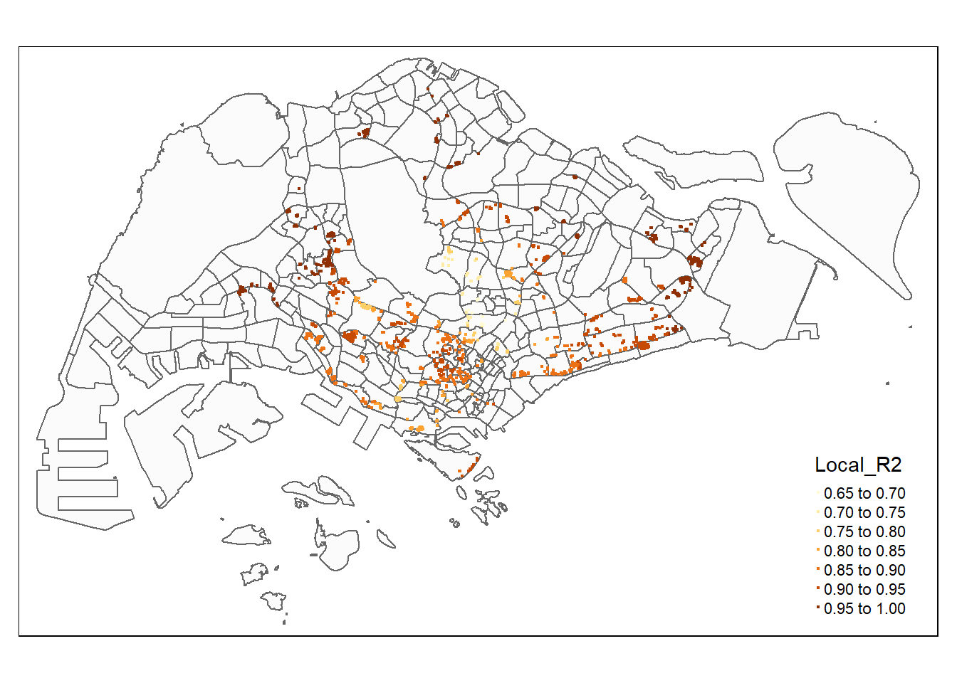
The code chunks below are used to create an interactive point symbol map.
tmap_mode("plot")
AREA_SQM_SE <- tm_shape(mpsz_svy21)+
  tm_polygons(alpha = 0.1) +
tm_shape(condo_resale.sf.adaptive) +
  tm_dots(col = "AREA_SQM_SE",
          border.col = "gray60",
          border.lwd = 1) +
  tm_view(set.zoom.limits = c(11,14))

AREA_SQM_TV <- tm_shape(mpsz_svy21)+
  tm_polygons(alpha = 0.1) +
tm_shape(condo_resale.sf.adaptive) +
  tm_dots(col = "AREA_SQM_TV",
          border.col = "gray60",
          border.lwd = 1) +
  tm_view(set.zoom.limits = c(11,14))

tmap_arrange(AREA_SQM_SE, AREA_SQM_TV,
             asp=1, ncol=2,
             sync = TRUE)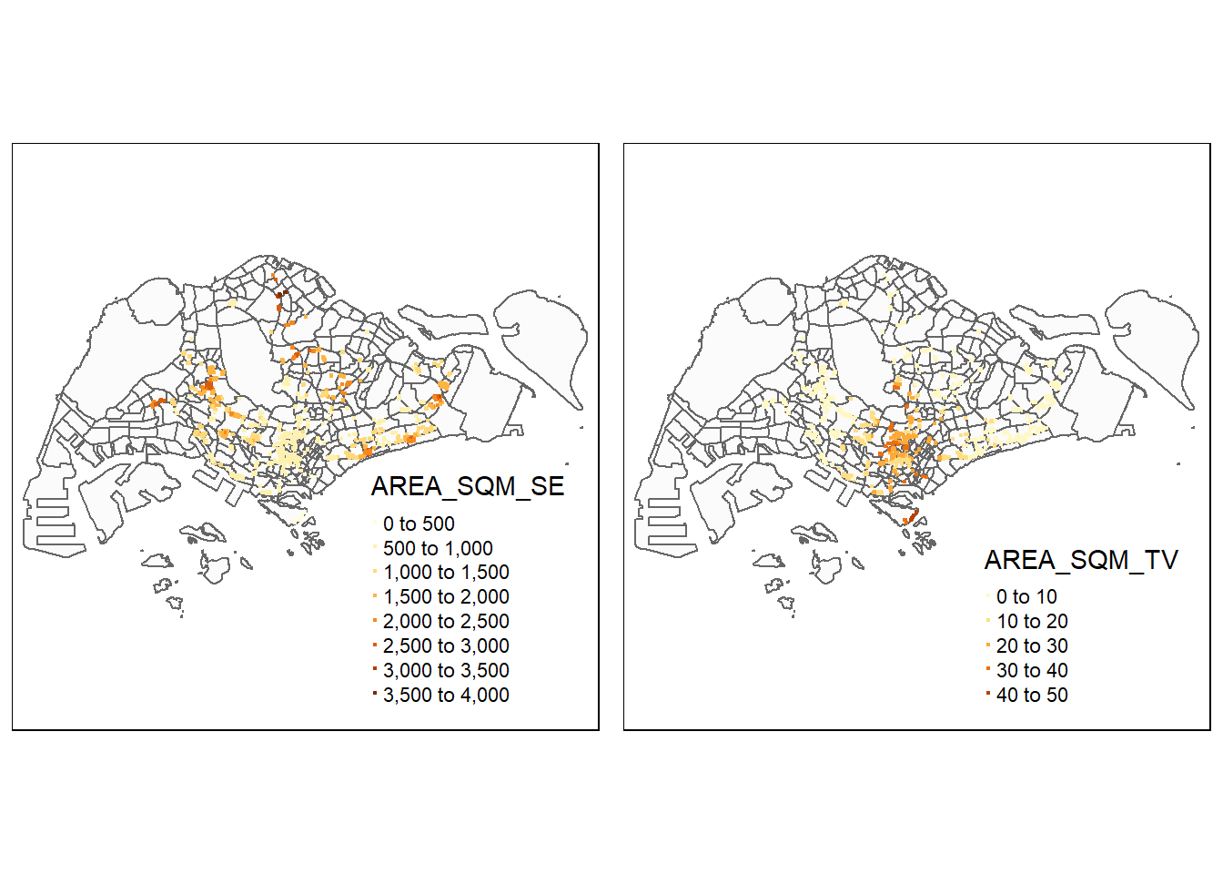
# correct the invalid geometry
fixed_geom <- sf::st_make_valid(mpsz_svy21[mpsz_svy21$REGION_N == "CENTRAL REGION", ])

tm_shape(fixed_geom[fixed_geom$REGION_N=="CENTRAL REGION", ])+
  tm_polygons()+
tm_shape(condo_resale.sf.adaptive) +
  tm_bubbles(col = "Local_R2",
           size = 0.15,
           border.col = "gray60",
           border.lwd = 1)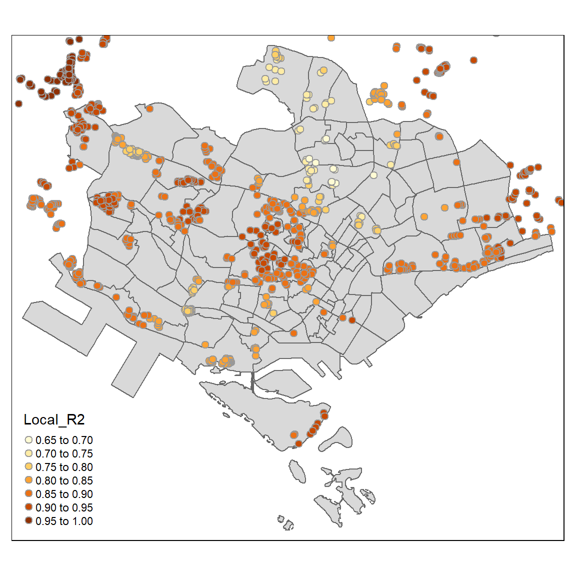
Gollini I, Lu B, Charlton M, Brunsdon C, Harris P (2015) “GWmodel: an R Package for exploring Spatial Heterogeneity using Geographically Weighted Models”. Journal of Statistical Software, 63(17):1-50, http://www.jstatsoft.org/v63/i17/
Lu B, Harris P, Charlton M, Brunsdon C (2014) “The GWmodel R Package: further topics for exploring Spatial Heterogeneity using Geographically Weighted Models”. Geo-spatial Information Science 17(2): 85-101, http://www.tandfonline.com/doi/abs/10.1080/1009502.2014.917453