Code
pacman::p_load(sf, spdep, tmap, tidyverse)Muhamad Ameer Noor
November 24, 2023
December 14, 2023
This exercise is a follow up of 2B exercise on exploring Global and Local Measures of Spatial Autocorrelation (GLSA) using the spdep package. Specifically, this 2C exercise will focus on Local Measures of Spatial Autocorrelation.
The new learning objectives includes: - Compute Local Indicator of Spatial Association (LISA) statistics to detect clusters and outliers. - Compute Getis-Ord’s Gi-statistics to identify hotspots or cold spots. - Visualize the analysis output using the tmap package.
Local measures of spatial autocorrelation, in contrast, focus on the relationships between each observation and its immediate surroundings. Instead of a single summary statistic, they provide specific scores for each observation, which help to understand more about the spatial structure in the data. These measures can tell us where specific clusters or outliers are located within the map. They are based on the same general principles as global measures but are more detailed, sometimes mathematically related to the global measures. Local Indicators of Spatial Association (LISAs) are a common example of this type of measure, offering a detailed view of spatial patterns and relationships at a local level. summarized from: Rey et al., 2020
load the packages
import, join, and visualize the data
Reading layer `Hunan' from data source `C:\ameernoor\ISSS624\data\geospatial' using driver `ESRI Shapefile'
Simple feature collection with 88 features and 7 fields
Geometry type: POLYGON
Dimension:     XY
Bounding box:  xmin: 108.7831 ymin: 24.6342 xmax: 114.2544 ymax: 30.12812
Geodetic CRS: WGS 84# import aspatial data
hunan2012 <- read_csv("../data/aspatial/Hunan_2012.csv")
# perform relational join
hunan <- left_join(hunan, hunan2012) %>%
select(1:4, 7, 15)
# visualize the data
equal <- tm_shape(hunan) +
tm_fill("GDPPC", n = 5, style = "equal") +
tm_borders(alpha = 0.5) +
tm_layout(main.title = "Equal interval classification", main.title.size = 1,
main.title.position = "center", legend.outside = TRUE,
legend.outside.position = "bottom")
quantile <- tm_shape(hunan) +
tm_fill("GDPPC", n = 5, style = "quantile") +
tm_borders(alpha = 0.5) +
tm_layout(main.title = "Equal quantile classification", main.title.size = 1,
main.title.position = "center", legend.outside = TRUE,
legend.outside.position = "bottom")
tmap_arrange(equal, quantile, asp=1, ncol=2)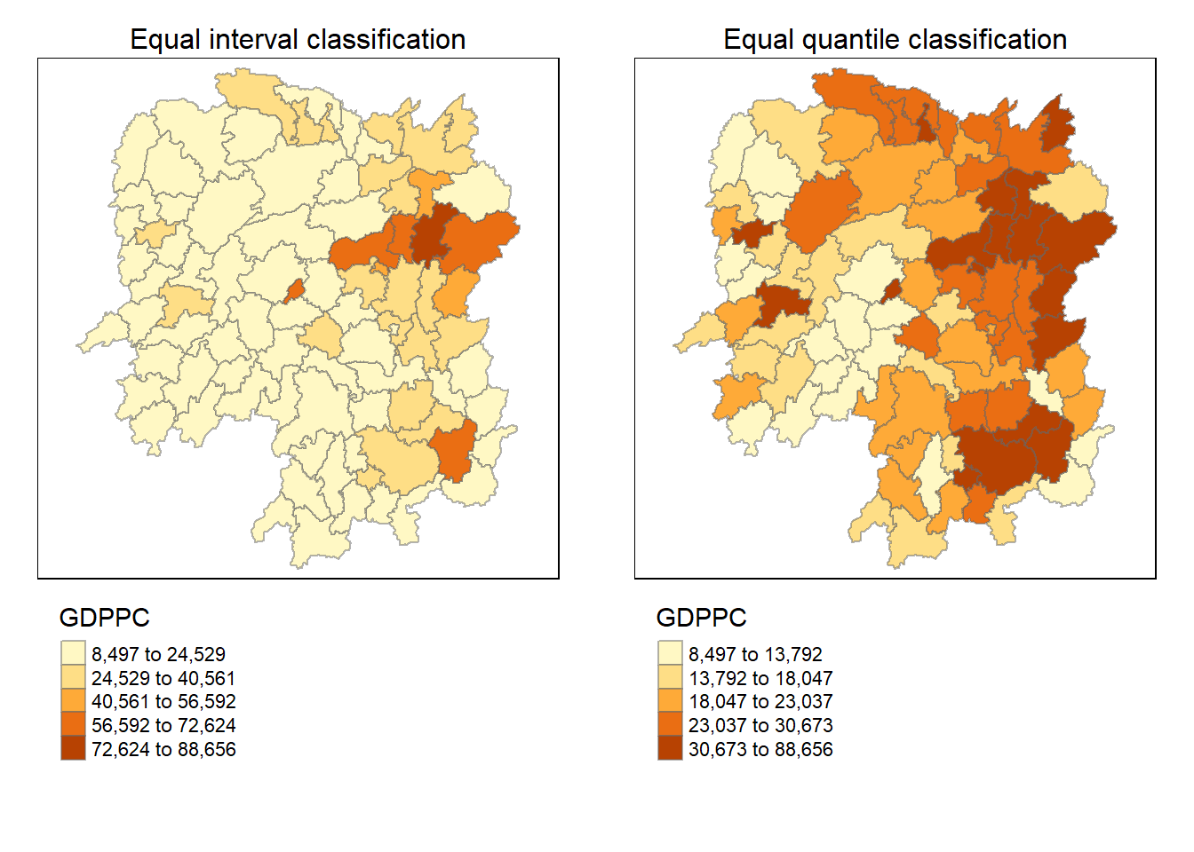
carry-over important variables from previous exercise
Local Indicators of Spatial Association (LISA) are statistical tools that help us identify clusters or outliers in the spatial distribution of a variable. Imagine studying cancer rates in different neighborhoods of a city; LISA would reveal whether there are areas with unusually high or low rates, indicating a spatial pattern beyond random chance. In this section, we’ll focus on applying LISA, particularly local Moran’s I, to detect clusters and outliers in the GDP per capita of Hunan Province, China, in 2012.
To calculate local Moran’s I, we use the localmoran() function of spdep package. This function computes various statistics, such as Ii, E.Ii, Var.Ii, Z.Ii, and Pr(), indicating the local spatial autocorrelation for each region.
            Ii          E.Ii       Var.Ii        Z.Ii Pr(z != E(Ii))
1 -0.001468468 -2.815006e-05 4.723841e-04 -0.06626904      0.9471636
2  0.025878173 -6.061953e-04 1.016664e-02  0.26266425      0.7928094
3 -0.011987646 -5.366648e-03 1.133362e-01 -0.01966705      0.9843090
4  0.001022468 -2.404783e-07 5.105969e-06  0.45259801      0.6508382
5  0.014814881 -6.829362e-05 1.449949e-03  0.39085814      0.6959021
6 -0.038793829 -3.860263e-04 6.475559e-03 -0.47728835      0.6331568
localmoran() function returns a matrix of values whose columns are: - Ii: the local Moran’s I statistics - E.Ii: the expectation of local moran statistic under the randomisation hypothesis - Var.Ii: the variance of local moran statistic under the randomisation hypothesis - Z.Ii:the standard deviate of local moran statistic - Pr(): the p-value of local moran statistic
The following code displays the content of the local Moran matrix by using printCoefmat().
                       Ii        E.Ii      Var.Ii        Z.Ii Pr.z....E.Ii..
Anhua         -2.2493e-02 -5.0048e-03  5.8235e-02 -7.2467e-02         0.9422
Anren         -3.9932e-01 -7.0111e-03  7.0348e-02 -1.4791e+00         0.1391
Anxiang       -1.4685e-03 -2.8150e-05  4.7238e-04 -6.6269e-02         0.9472
Baojing        3.4737e-01 -5.0089e-03  8.3636e-02  1.2185e+00         0.2230
Chaling        2.0559e-02 -9.6812e-04  2.7711e-02  1.2932e-01         0.8971
Changning     -2.9868e-05 -9.0010e-09  1.5105e-07 -7.6828e-02         0.9388
Changsha       4.9022e+00 -2.1348e-01  2.3194e+00  3.3590e+00         0.0008
Chengbu        7.3725e-01 -1.0534e-02  2.2132e-01  1.5895e+00         0.1119
Chenxi         1.4544e-01 -2.8156e-03  4.7116e-02  6.8299e-01         0.4946
Cili           7.3176e-02 -1.6747e-03  4.7902e-02  3.4200e-01         0.7324
Dao            2.1420e-01 -2.0824e-03  4.4123e-02  1.0297e+00         0.3032
Dongan         1.5210e-01 -6.3485e-04  1.3471e-02  1.3159e+00         0.1882
Dongkou        5.2918e-01 -6.4461e-03  1.0748e-01  1.6338e+00         0.1023
Fenghuang      1.8013e-01 -6.2832e-03  1.3257e-01  5.1198e-01         0.6087
Guidong       -5.9160e-01 -1.3086e-02  3.7003e-01 -9.5104e-01         0.3416
Guiyang        1.8240e-01 -3.6908e-03  3.2610e-02  1.0305e+00         0.3028
Guzhang        2.8466e-01 -8.5054e-03  1.4152e-01  7.7931e-01         0.4358
Hanshou        2.5878e-02 -6.0620e-04  1.0167e-02  2.6266e-01         0.7928
Hengdong       9.9964e-03 -4.9063e-04  6.7742e-03  1.2742e-01         0.8986
Hengnan        2.8064e-02 -3.2160e-04  3.7597e-03  4.6294e-01         0.6434
Hengshan      -5.8201e-03 -3.0437e-05  5.1076e-04 -2.5618e-01         0.7978
Hengyang       6.2997e-02 -1.3046e-03  2.1865e-02  4.3486e-01         0.6637
Hongjiang      1.8790e-01 -2.3019e-03  3.1725e-02  1.0678e+00         0.2856
Huarong       -1.5389e-02 -1.8667e-03  8.1030e-02 -4.7503e-02         0.9621
Huayuan        8.3772e-02 -8.5569e-04  2.4495e-02  5.4072e-01         0.5887
Huitong        2.5997e-01 -5.2447e-03  1.1077e-01  7.9685e-01         0.4255
Jiahe         -1.2431e-01 -3.0550e-03  5.1111e-02 -5.3633e-01         0.5917
Jianghua       2.8651e-01 -3.8280e-03  8.0968e-02  1.0204e+00         0.3076
Jiangyong      2.4337e-01 -2.7082e-03  1.1746e-01  7.1800e-01         0.4728
Jingzhou       1.8270e-01 -8.5106e-04  2.4363e-02  1.1759e+00         0.2396
Jinshi        -1.1988e-02 -5.3666e-03  1.1334e-01 -1.9667e-02         0.9843
Jishou        -2.8680e-01 -2.6305e-03  4.4028e-02 -1.3543e+00         0.1756
Lanshan        6.3334e-02 -9.6365e-04  2.0441e-02  4.4972e-01         0.6529
Leiyang        1.1581e-02 -1.4948e-04  2.5082e-03  2.3422e-01         0.8148
Lengshuijiang -1.7903e+00 -8.2129e-02  2.1598e+00 -1.1623e+00         0.2451
Li             1.0225e-03 -2.4048e-07  5.1060e-06  4.5260e-01         0.6508
Lianyuan      -1.4672e-01 -1.8983e-03  1.9145e-02 -1.0467e+00         0.2952
Liling         1.3774e+00 -1.5097e-02  4.2601e-01  2.1335e+00         0.0329
Linli          1.4815e-02 -6.8294e-05  1.4499e-03  3.9086e-01         0.6959
Linwu         -2.4621e-03 -9.0703e-06  1.9258e-04 -1.7676e-01         0.8597
Linxiang       6.5904e-02 -2.9028e-03  2.5470e-01  1.3634e-01         0.8916
Liuyang        3.3688e+00 -7.7502e-02  1.5180e+00  2.7972e+00         0.0052
Longhui        8.0801e-01 -1.1377e-02  1.5538e-01  2.0787e+00         0.0376
Longshan       7.5663e-01 -1.1100e-02  3.1449e-01  1.3690e+00         0.1710
Luxi           1.8177e-01 -2.4855e-03  3.4249e-02  9.9561e-01         0.3194
Mayang         2.1852e-01 -5.8773e-03  9.8049e-02  7.1663e-01         0.4736
Miluo          1.8704e+00 -1.6927e-02  2.7925e-01  3.5715e+00         0.0004
Nan           -9.5789e-03 -4.9497e-04  6.8341e-03 -1.0988e-01         0.9125
Ningxiang      1.5607e+00 -7.3878e-02  8.0012e-01  1.8274e+00         0.0676
Ningyuan       2.0910e-01 -7.0884e-03  8.2306e-02  7.5356e-01         0.4511
Pingjiang     -9.8964e-01 -2.6457e-03  5.6027e-02 -4.1698e+00         0.0000
Qidong         1.1806e-01 -2.1207e-03  2.4747e-02  7.6396e-01         0.4449
Qiyang         6.1966e-02 -7.3374e-04  8.5743e-03  6.7712e-01         0.4983
Rucheng       -3.6992e-01 -8.8999e-03  2.5272e-01 -7.1814e-01         0.4727
Sangzhi        2.5053e-01 -4.9470e-03  6.8000e-02  9.7972e-01         0.3272
Shaodong      -3.2659e-02 -3.6592e-05  5.0546e-04 -1.4510e+00         0.1468
Shaoshan       2.1223e+00 -5.0227e-02  1.3668e+00  1.8583e+00         0.0631
Shaoyang       5.9499e-01 -1.1253e-02  1.3012e-01  1.6807e+00         0.0928
Shimen        -3.8794e-02 -3.8603e-04  6.4756e-03 -4.7729e-01         0.6332
Shuangfeng     9.2835e-03 -2.2867e-03  3.1516e-02  6.5174e-02         0.9480
Shuangpai      8.0591e-02 -3.1366e-04  8.9838e-03  8.5358e-01         0.3933
Suining        3.7585e-01 -3.5933e-03  4.1870e-02  1.8544e+00         0.0637
Taojiang      -2.5394e-01 -1.2395e-03  1.4477e-02 -2.1002e+00         0.0357
Taoyuan        1.4729e-02 -1.2039e-04  8.5103e-04  5.0903e-01         0.6107
Tongdao        4.6482e-01 -6.9870e-03  1.9879e-01  1.0582e+00         0.2900
Wangcheng      4.4220e+00 -1.1067e-01  1.3596e+00  3.8873e+00         0.0001
Wugang         7.1003e-01 -7.8144e-03  1.0710e-01  2.1935e+00         0.0283
Xiangtan       2.4530e-01 -3.6457e-04  3.2319e-03  4.3213e+00         0.0000
Xiangxiang     2.6271e-01 -1.2703e-03  2.1290e-02  1.8092e+00         0.0704
Xiangyin       5.4525e-01 -4.7442e-03  7.9236e-02  1.9539e+00         0.0507
Xinhua         1.1810e-01 -6.2649e-03  8.6001e-02  4.2409e-01         0.6715
Xinhuang       1.5725e-01 -4.1820e-03  3.6648e-01  2.6667e-01         0.7897
Xinning        6.8928e-01 -9.6674e-03  2.0328e-01  1.5502e+00         0.1211
Xinshao        5.7578e-02 -8.5932e-03  1.1769e-01  1.9289e-01         0.8470
Xintian       -7.4050e-03 -5.1493e-03  1.0877e-01 -6.8395e-03         0.9945
Xupu           3.2406e-01 -5.7468e-03  5.7735e-02  1.3726e+00         0.1699
Yanling       -6.9021e-02 -5.9211e-04  9.9306e-03 -6.8667e-01         0.4923
Yizhang       -2.6844e-01 -2.2463e-03  4.7588e-02 -1.2202e+00         0.2224
Yongshun       6.3064e-01 -1.1350e-02  1.8830e-01  1.4795e+00         0.1390
Yongxing       4.3411e-01 -9.0735e-03  1.5088e-01  1.1409e+00         0.2539
You            7.8750e-02 -7.2728e-03  1.2116e-01  2.4714e-01         0.8048
Yuanjiang      2.0004e-04 -1.7760e-04  2.9798e-03  6.9181e-03         0.9945
Yuanling       8.7298e-03 -2.2981e-06  2.3221e-05  1.8121e+00         0.0700
Yueyang        4.1189e-02 -1.9768e-04  2.3113e-03  8.6085e-01         0.3893
Zhijiang       1.0476e-01 -7.8123e-04  1.3100e-02  9.2214e-01         0.3565
Zhongfang     -2.2685e-01 -2.1455e-03  3.5927e-02 -1.1855e+00         0.2358
Zhuzhou        3.2864e-01 -5.2432e-04  7.2391e-03  3.8688e+00         0.0001
Zixing -7.6849e-01 -8.8210e-02 9.4057e-01 -7.0144e-01 0.4830To visualize the local Moran’s I, we append the local Moran’s I dataframe to the hunan SpatialPolygonDataFrame, creating hunan.localMI. We can then use tmap to create choropleth maps.
the code below uses tmap to plot a choropleth map of local Moran’s I values.
Considering both Ii values and their p-values is essential. The code chunk below creates a choropleth map of Moran’s I p-values.
For a comprehensive interpretation, it’s beneficial to plot both the local Moran’s I values and their corresponding p-values side by side.
localMI.map <- tm_shape(hunan.localMI) +
  tm_fill(col = "Ii",
          style = "pretty",
          title = "local moran statistics") +
  tm_borders(alpha = 0.5)

pvalue.map <- tm_shape(hunan.localMI) +
  tm_fill(col = "Pr.Ii",
          breaks=c(-Inf, 0.001, 0.01, 0.05, 0.1, Inf),
          palette="-Blues",
          title = "local Moran's I p-values") +
  tm_borders(alpha = 0.5)

tmap_arrange(localMI.map, pvalue.map, asp=1, ncol=2)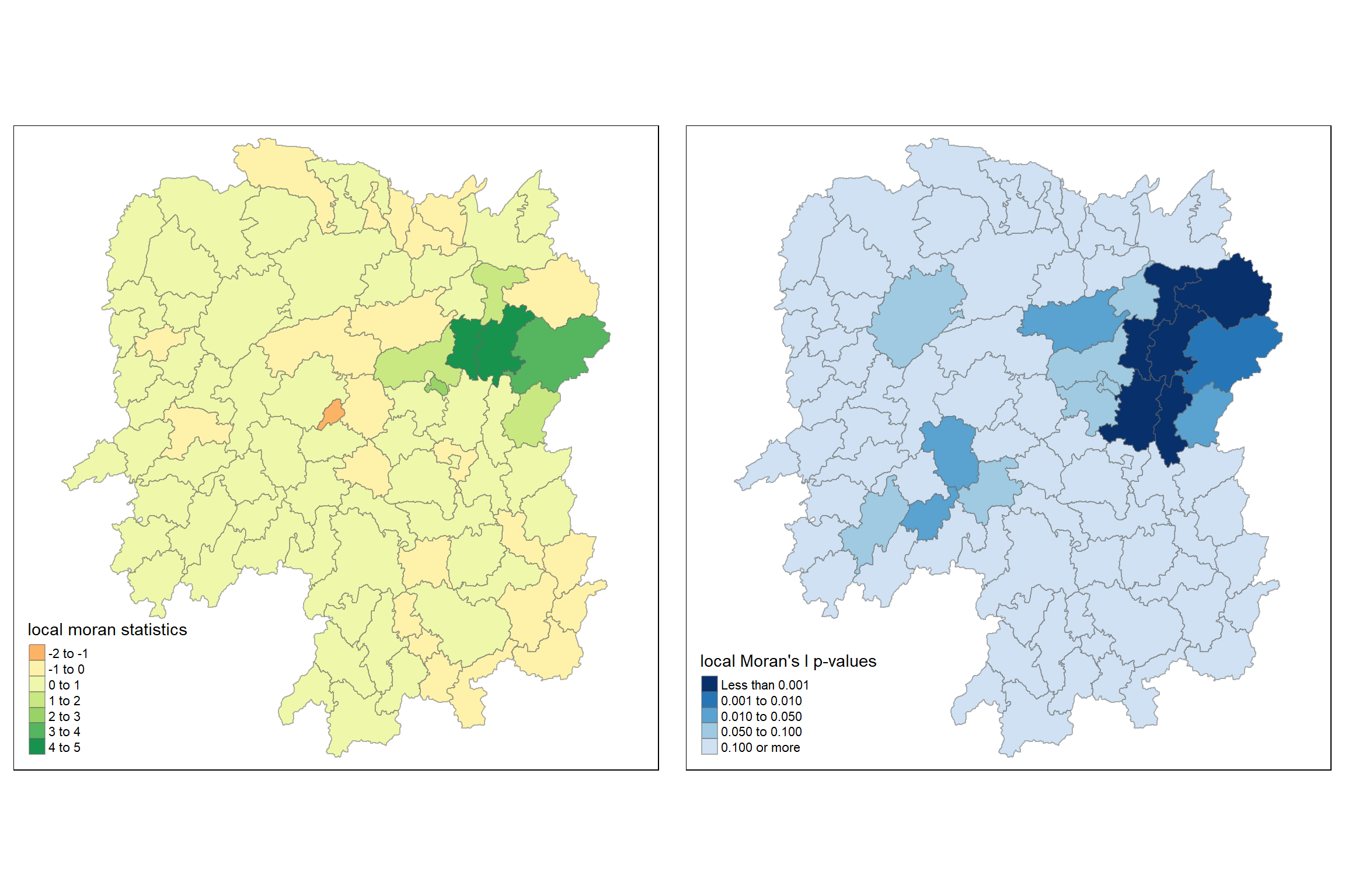
The LISA Cluster Map helps us identify significant spatial clusters by color-coding areas based on their type of spatial autocorrelation. To generate this map, we start by plotting the Moran scatterplot.
A LISA (Local Indicators of Spatial Association) Cluster Map is a tool used in geography and spatial analysis to identify areas of significant spatial autocorrelation in a dataset. It visually represents regions where observed values (like population density, temperature, etc.) are either similar or dissimilar to their neighboring areas. The map highlights clusters of high values near high values (high-high), low values near low values (low-low), and areas where high values are near low values (high-low) and vice versa. This visualization helps to easily identify areas of similar or dissimilar values and understand spatial patterns and relationships within the data. In essence, it’s a way to see where certain types of values are grouped together on a map.
The Moran scatterplot illustrates how the values of a variable at each location relate to the average values at neighboring locations. The code below uses moran.plot() from the spdep package to create this plot for the GDPPC.
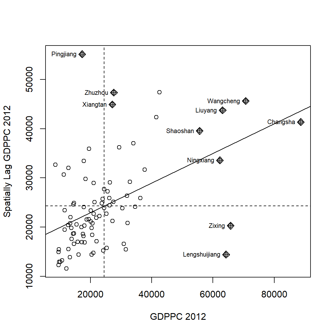
The plot is divided into four quadrants. The top right quadrant represents areas with high GDPPC surrounded by areas with average GDPPC – these are the high-high locations.
To enhance the analysis, we standardize the GDPPC variable using the scale() function. Then, we plot the Moran scatterplot again.
The as.vector() added to the end is to make sure that the data type we get is a vector that map neatly into the dataframe.
The following code prepares the LISA cluster map by categorizing areas into low-low, low-high, high-low, high-high, or insignificant clusters, and plot it into a map.
# Create an empty vector to store the quadrant information for each area
quadrant <- vector(mode="numeric",length=nrow(localMI))

# Calculate the spatially lagged variable (DV) by subtracting the mean from the lagged GDPPC
hunan$lag_GDPPC <- lag.listw(rswm_q, hunan$GDPPC)
DV <- hunan$lag_GDPPC - mean(hunan$lag_GDPPC)

# Calculate the local Moran's I values (LM_I) by subtracting the mean from the original values
LM_I <- localMI[,1] - mean(localMI[,1])

# Set the significance level for the local Moran's I
signif <- 0.05

# Categorize areas into different quadrants based on their DV and LM_I values
quadrant[DV < 0 & LM_I > 0] <- 1  # Low values surrounded by high values (low-high)
quadrant[DV > 0 & LM_I < 0] <- 2  # High values surrounded by low values (high-low)
quadrant[DV < 0 & LM_I < 0] <- 3  # Low values surrounded by low values (low-low)
quadrant[DV > 0 & LM_I > 0] <- 4  # High values surrounded by high values (high-high)

# Identify areas with non-significant Moran's I values and label them as 0
quadrant[localMI[,5] > signif] <- 0


hunan.localMI$quadrant <- quadrant
colors <- c("#ffffff", "#2c7bb6", "#abd9e9", "#fdae61", "#d7191c")
clusters <- c("insignificant", "low-low", "low-high", "high-low", "high-high")

tm_shape(hunan.localMI) +
  tm_fill(col = "quadrant",
          style = "cat",
          palette = colors[c(sort(unique(quadrant)))+1],
          labels = clusters[c(sort(unique(quadrant)))+1],
          popup.vars = c("")) +
  tm_view(set.zoom.limits = c(11,17)) +
  tm_borders(alpha=0.5)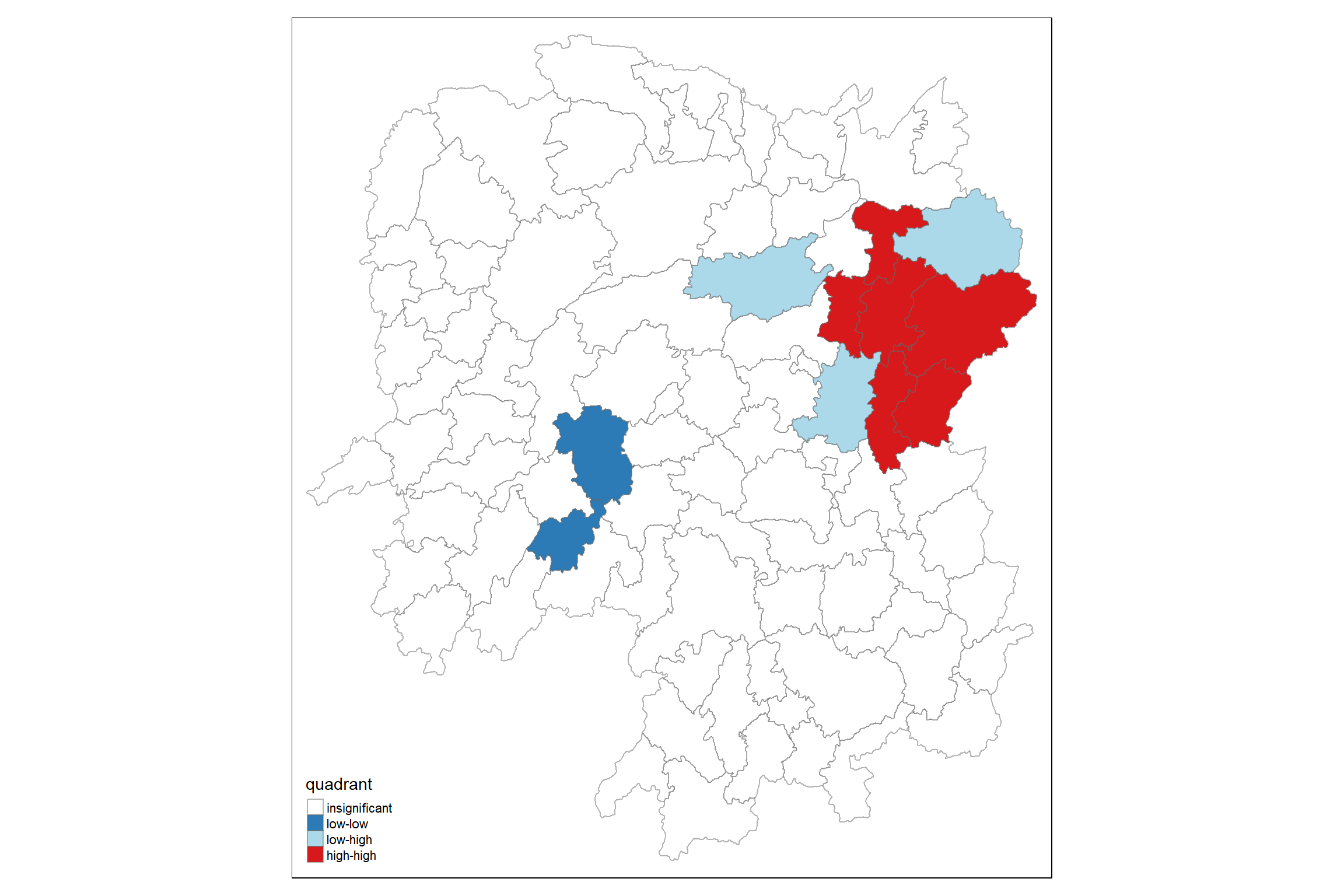
For effective interpretation, it is better to plot both the local Moran’s I values map and its corresponding p-values map next to each other.
The code chunk below will be used to create such visualisation.
gdppc <- qtm(hunan, "GDPPC")

hunan.localMI$quadrant <- quadrant
colors <- c("#ffffff", "#2c7bb6", "#abd9e9", "#fdae61", "#d7191c")
clusters <- c("insignificant", "low-low", "low-high", "high-low", "high-high")

LISAmap <- tm_shape(hunan.localMI) +
  tm_fill(col = "quadrant",
          style = "cat",
          palette = colors[c(sort(unique(quadrant)))+1],
          labels = clusters[c(sort(unique(quadrant)))+1],
          popup.vars = c("")) +
  tm_view(set.zoom.limits = c(11,17)) +
  tm_borders(alpha=0.5)

tmap_arrange(gdppc, LISAmap,
             asp=1, ncol=2)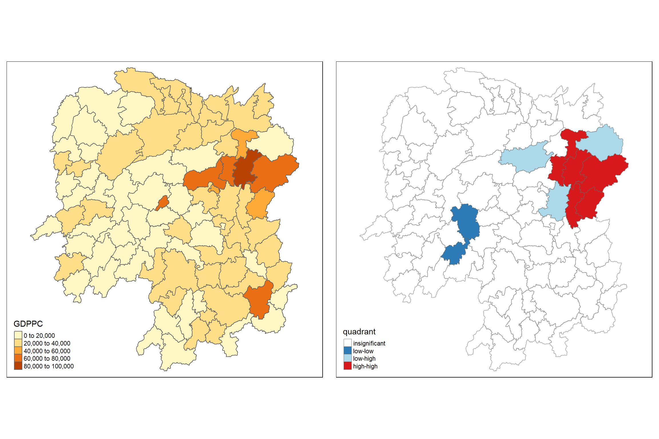
We can also include the local Moran’s I map and p-value map as shown below for easy comparison.

The LISA maps show significant spatial clustering of economic activity. Counties with a high GDP per Capita geographically clustered together indicates positive spatial autocorrelation. Conversely, areas with low Moran’s I values (orange) indicate counties with lower GDP per Capita that may be surrounded by higher-income counties. But, previous data processing section shows that some of the negative area might actually be richer, but the technical calculation averaged it down.
In addition to finding clusters and outliers, localized spatial statistics can help identify hot spot and cold spot areas. The term ‘hot spot’ generally refers to a region or value that is higher relative to its surroundings. The Getis and Ord’s G-statistics is a spatial statistical method that detects spatial anomalies by examining neighbors within a specified proximity to identify where either high or low values cluster spatially. Statistically significant hot spots are areas with high values where neighboring areas also exhibit high values. The analysis involves three steps: deriving a spatial weight matrix, computing Gi statistics, and mapping Gi statistics.
Initially, we need to define new neighbors based on distance rather than shared borders, which was considered in spatial autocorrelation. Two types of distance-based proximity matrices are fixed distance weight matrix and adaptive distance weight matrix.
First, we need points associated with each polygon, and to achieve this, we use the st_centroid() function. Longitude and latitude values are extracted separately and combined into a coordinate matrix.
We determine the upper limit for the distance band by finding the k nearest neighbors for each point and calculating the distance between them.
   Min. 1st Qu.  Median    Mean 3rd Qu.    Max.
  24.79   32.57   38.01   39.07   44.52   61.79
The summary indicates the largest first nearest neighbor distance is 61.79 km, setting this as the upper threshold ensures all units have at least one neighbor.
Now, we calculate the distance weight matrix bt using a fixed distance of 62 km and dnearneigh() function
Neighbour list object:
Number of regions: 88
Number of nonzero links: 324
Percentage nonzero weights: 4.183884
Average number of links: 3.681818
Then, we convert the neighbor object into a spatial weights object named wm62_lw using nb2listw().
Characteristics of weights list object:
Neighbour list object:
Number of regions: 88
Number of nonzero links: 324
Percentage nonzero weights: 4.183884
Average number of links: 3.681818
Link number distribution:

 1  2  3  4  5  6
 6 15 14 26 20  7
6 least connected regions:
6 15 30 32 56 65 with 1 link
7 most connected regions:
21 28 35 45 50 52 82 with 6 links

Weights style: B
Weights constants summary:
   n   nn  S0  S1   S2
B 88 7744 324 648 5440Fixed distance weight matrices tend to assign more neighbors to densely settled areas and fewer neighbors to less densely settled areas. To control the number of neighbors directly, we use k-nearest neighbors and specify k.
Neighbour list object:
Number of regions: 88
Number of nonzero links: 704
Percentage nonzero weights: 9.090909
Average number of links: 8
Non-symmetric neighbours list
Then, we convert the neighbor object into a spatial weights object
Characteristics of weights list object:
Neighbour list object:
Number of regions: 88
Number of nonzero links: 704
Percentage nonzero weights: 9.090909
Average number of links: 8
Non-symmetric neighbours list
Link number distribution:

 8
88
88 least connected regions:
1 2 3 4 5 6 7 8 9 10 11 12 13 14 15 16 17 18 19 20 21 22 23 24 25 26 27 28 29 30 31 32 33 34 35 36 37 38 39 40 41 42 43 44 45 46 47 48 49 50 51 52 53 54 55 56 57 58 59 60 61 62 63 64 65 66 67 68 69 70 71 72 73 74 75 76 77 78 79 80 81 82 83 84 85 86 87 88 with 8 links
88 most connected regions:
1 2 3 4 5 6 7 8 9 10 11 12 13 14 15 16 17 18 19 20 21 22 23 24 25 26 27 28 29 30 31 32 33 34 35 36 37 38 39 40 41 42 43 44 45 46 47 48 49 50 51 52 53 54 55 56 57 58 59 60 61 62 63 64 65 66 67 68 69 70 71 72 73 74 75 76 77 78 79 80 81 82 83 84 85 86 87 88 with 8 links

Weights style: B
Weights constants summary:
   n   nn  S0   S1    S2
B 88 7744 704 1300 23014Gi statistics help us find areas with unusually high or low values compared to their neighbors
The first code chunk computes Gi statistics using a fixed distance weight matrix (wm62_lw). The resulting Gi values are Z-scores, where greater values indicate stronger clustering intensity. We then join these Gi values to the original data frame for visualization.
 [1]  0.436075843 -0.265505650 -0.073033665  0.413017033  0.273070579
 [6] -0.377510776  2.863898821  2.794350420  5.216125401  0.228236603
[11]  0.951035346 -0.536334231  0.176761556  1.195564020 -0.033020610
[16]  1.378081093 -0.585756761 -0.419680565  0.258805141  0.012056111
[21] -0.145716531 -0.027158687 -0.318615290 -0.748946051 -0.961700582
[26] -0.796851342 -1.033949773 -0.460979158 -0.885240161 -0.266671512
[31] -0.886168613 -0.855476971 -0.922143185 -1.162328599  0.735582222
[36] -0.003358489 -0.967459309 -1.259299080 -1.452256513 -1.540671121
[41] -1.395011407 -1.681505286 -1.314110709 -0.767944457 -0.192889342
[46]  2.720804542  1.809191360 -1.218469473 -0.511984469 -0.834546363
[51] -0.908179070 -1.541081516 -1.192199867 -1.075080164 -1.631075961
[56] -0.743472246  0.418842387  0.832943753 -0.710289083 -0.449718820
[61] -0.493238743 -1.083386776  0.042979051  0.008596093  0.136337469
[66]  2.203411744  2.690329952  4.453703219 -0.340842743 -0.129318589
[71]  0.737806634 -1.246912658  0.666667559  1.088613505 -0.985792573
[76]  1.233609606 -0.487196415  1.626174042 -1.060416797  0.425361422
[81] -0.837897118 -0.314565243  0.371456331  4.424392623 -0.109566928
[86]  1.364597995 -1.029658605 -0.718000620
attr(,"internals")
               Gi      E(Gi)        V(Gi)        Z(Gi) Pr(z != E(Gi))
 [1,] 0.064192949 0.05747126 2.375922e-04  0.436075843   6.627817e-01
 [2,] 0.042300020 0.04597701 1.917951e-04 -0.265505650   7.906200e-01
 [3,] 0.044961480 0.04597701 1.933486e-04 -0.073033665   9.417793e-01
 [4,] 0.039475779 0.03448276 1.461473e-04  0.413017033   6.795941e-01
 [5,] 0.049767939 0.04597701 1.927263e-04  0.273070579   7.847990e-01
 [6,] 0.008825335 0.01149425 4.998177e-05 -0.377510776   7.057941e-01
 [7,] 0.050807266 0.02298851 9.435398e-05  2.863898821   4.184617e-03
 [8,] 0.083966739 0.04597701 1.848292e-04  2.794350420   5.200409e-03
 [9,] 0.115751554 0.04597701 1.789361e-04  5.216125401   1.827045e-07
[10,] 0.049115587 0.04597701 1.891013e-04  0.228236603   8.194623e-01
[11,] 0.045819180 0.03448276 1.420884e-04  0.951035346   3.415864e-01
[12,] 0.049183846 0.05747126 2.387633e-04 -0.536334231   5.917276e-01
[13,] 0.048429181 0.04597701 1.924532e-04  0.176761556   8.596957e-01
[14,] 0.034733752 0.02298851 9.651140e-05  1.195564020   2.318667e-01
[15,] 0.011262043 0.01149425 4.945294e-05 -0.033020610   9.736582e-01
[16,] 0.065131196 0.04597701 1.931870e-04  1.378081093   1.681783e-01
[17,] 0.027587075 0.03448276 1.385862e-04 -0.585756761   5.580390e-01
[18,] 0.029409313 0.03448276 1.461397e-04 -0.419680565   6.747188e-01
[19,] 0.061466754 0.05747126 2.383385e-04  0.258805141   7.957856e-01
[20,] 0.057656917 0.05747126 2.371303e-04  0.012056111   9.903808e-01
[21,] 0.066518379 0.06896552 2.820326e-04 -0.145716531   8.841452e-01
[22,] 0.045599896 0.04597701 1.928108e-04 -0.027158687   9.783332e-01
[23,] 0.030646753 0.03448276 1.449523e-04 -0.318615290   7.500183e-01
[24,] 0.035635552 0.04597701 1.906613e-04 -0.748946051   4.538897e-01
[25,] 0.032606647 0.04597701 1.932888e-04 -0.961700582   3.362000e-01
[26,] 0.035001352 0.04597701 1.897172e-04 -0.796851342   4.255374e-01
[27,] 0.012746354 0.02298851 9.812587e-05 -1.033949773   3.011596e-01
[28,] 0.061287917 0.06896552 2.773884e-04 -0.460979158   6.448136e-01
[29,] 0.014277403 0.02298851 9.683314e-05 -0.885240161   3.760271e-01
[30,] 0.009622875 0.01149425 4.924586e-05 -0.266671512   7.897221e-01
[31,] 0.014258398 0.02298851 9.705244e-05 -0.886168613   3.755267e-01
[32,] 0.005453443 0.01149425 4.986245e-05 -0.855476971   3.922871e-01
[33,] 0.043283712 0.05747126 2.367109e-04 -0.922143185   3.564539e-01
[34,] 0.020763514 0.03448276 1.393165e-04 -1.162328599   2.451020e-01
[35,] 0.081261843 0.06896552 2.794398e-04  0.735582222   4.619850e-01
[36,] 0.057419907 0.05747126 2.338437e-04 -0.003358489   9.973203e-01
[37,] 0.013497133 0.02298851 9.624821e-05 -0.967459309   3.333145e-01
[38,] 0.019289310 0.03448276 1.455643e-04 -1.259299080   2.079223e-01
[39,] 0.025996272 0.04597701 1.892938e-04 -1.452256513   1.464303e-01
[40,] 0.016092694 0.03448276 1.424776e-04 -1.540671121   1.233968e-01
[41,] 0.035952614 0.05747126 2.379439e-04 -1.395011407   1.630124e-01
[42,] 0.031690963 0.05747126 2.350604e-04 -1.681505286   9.266481e-02
[43,] 0.018750079 0.03448276 1.433314e-04 -1.314110709   1.888090e-01
[44,] 0.015449080 0.02298851 9.638666e-05 -0.767944457   4.425202e-01
[45,] 0.065760689 0.06896552 2.760533e-04 -0.192889342   8.470456e-01
[46,] 0.098966900 0.05747126 2.326002e-04  2.720804542   6.512325e-03
[47,] 0.085415780 0.05747126 2.385746e-04  1.809191360   7.042128e-02
[48,] 0.038816536 0.05747126 2.343951e-04 -1.218469473   2.230456e-01
[49,] 0.038931873 0.04597701 1.893501e-04 -0.511984469   6.086619e-01
[50,] 0.055098610 0.06896552 2.760948e-04 -0.834546363   4.039732e-01
[51,] 0.033405005 0.04597701 1.916312e-04 -0.908179070   3.637836e-01
[52,] 0.043040784 0.06896552 2.829941e-04 -1.541081516   1.232969e-01
[53,] 0.011297699 0.02298851 9.615920e-05 -1.192199867   2.331829e-01
[54,] 0.040968457 0.05747126 2.356318e-04 -1.075080164   2.823388e-01
[55,] 0.023629663 0.04597701 1.877170e-04 -1.631075961   1.028743e-01
[56,] 0.006281129 0.01149425 4.916619e-05 -0.743472246   4.571958e-01
[57,] 0.063918654 0.05747126 2.369553e-04  0.418842387   6.753313e-01
[58,] 0.070325003 0.05747126 2.381374e-04  0.832943753   4.048765e-01
[59,] 0.025947288 0.03448276 1.444058e-04 -0.710289083   4.775249e-01
[60,] 0.039752578 0.04597701 1.915656e-04 -0.449718820   6.529132e-01
[61,] 0.049934283 0.05747126 2.334965e-04 -0.493238743   6.218439e-01
[62,] 0.030964195 0.04597701 1.920248e-04 -1.083386776   2.786368e-01
[63,] 0.058129184 0.05747126 2.343319e-04  0.042979051   9.657182e-01
[64,] 0.046096514 0.04597701 1.932637e-04  0.008596093   9.931414e-01
[65,] 0.012459080 0.01149425 5.008051e-05  0.136337469   8.915545e-01
[66,] 0.091447733 0.05747126 2.377744e-04  2.203411744   2.756574e-02
[67,] 0.049575872 0.02298851 9.766513e-05  2.690329952   7.138140e-03
[68,] 0.107907212 0.04597701 1.933581e-04  4.453703219   8.440175e-06
[69,] 0.019616151 0.02298851 9.789454e-05 -0.340842743   7.332220e-01
[70,] 0.032923393 0.03448276 1.454032e-04 -0.129318589   8.971056e-01
[71,] 0.030317663 0.02298851 9.867859e-05  0.737806634   4.606320e-01
[72,] 0.019437582 0.03448276 1.455870e-04 -1.246912658   2.124295e-01
[73,] 0.055245460 0.04597701 1.932838e-04  0.666667559   5.049845e-01
[74,] 0.074278054 0.05747126 2.383538e-04  1.088613505   2.763244e-01
[75,] 0.013269580 0.02298851 9.719982e-05 -0.985792573   3.242349e-01
[76,] 0.049407829 0.03448276 1.463785e-04  1.233609606   2.173484e-01
[77,] 0.028605749 0.03448276 1.455139e-04 -0.487196415   6.261191e-01
[78,] 0.039087662 0.02298851 9.801040e-05  1.626174042   1.039126e-01
[79,] 0.031447120 0.04597701 1.877464e-04 -1.060416797   2.889550e-01
[80,] 0.064005294 0.05747126 2.359641e-04  0.425361422   6.705732e-01
[81,] 0.044606529 0.05747126 2.357330e-04 -0.837897118   4.020885e-01
[82,] 0.063700493 0.06896552 2.801427e-04 -0.314565243   7.530918e-01
[83,] 0.051142205 0.04597701 1.933560e-04  0.371456331   7.102977e-01
[84,] 0.102121112 0.04597701 1.610278e-04  4.424392623   9.671399e-06
[85,] 0.021901462 0.02298851 9.843172e-05 -0.109566928   9.127528e-01
[86,] 0.064931813 0.04597701 1.929430e-04  1.364597995   1.723794e-01
[87,] 0.031747344 0.04597701 1.909867e-04 -1.029658605   3.031703e-01
[88,] 0.015893319 0.02298851 9.765131e-05 -0.718000620   4.727569e-01
attr(,"cluster")
 [1] Low  Low  High High High High High High High Low  Low  High Low  Low  Low
[16] High High High High Low  High High Low  Low  High Low  Low  Low  Low  Low
[31] Low  Low  Low  High Low  Low  Low  Low  Low  Low  High Low  Low  Low  Low
[46] High High Low  Low  Low  Low  High Low  Low  Low  Low  Low  High Low  Low
[61] Low  Low  Low  High High High Low  High Low  Low  High Low  High High Low
[76] High Low  Low  Low  Low  Low  Low  High High Low  High Low  Low
Levels: Low High
attr(,"gstari")
[1] FALSE
attr(,"call")
localG(x = hunan$GDPPC, listw = wm62_lw)
attr(,"class")
[1] "localG"
The Gi statistics, represented as Z-scores, are now linked to the original data frame. We visualize these values on a map using a choropleth map, where colors indicate the intensity and direction of clustering.
# Combine the Gi statistics with the original data frame 'hunan'
# Convert the Gi vector ('gi.fixed') to a matrix and bind it to the original data frame ('hunan')
# Rename the newly added column to 'gstat_fixed'
hunan.gi <- cbind(hunan, as.matrix(gi.fixed)) %>%
  rename(gstat_fixed = as.matrix.gi.fixed.)

# Create a quick thematic map (qtm) of the original data frame ('hunan') for GDP per capita ('GDPPC')
gdppc <- qtm(hunan, "GDPPC")

# Create a thematic map (Gimap) for Gi statistics using the 'tm' package
# Shape the map based on the combined data frame ('hunan.gi')
Gimap <-tm_shape(hunan.gi) +
  # Fill the map with colors based on 'gstat_fixed' column
  tm_fill(col = "gstat_fixed",
          # Use the 'pretty' style for color breaks
          style = "pretty",
          # Choose the RdBu color palette
          palette="-RdBu",
          # Set the title for the legend
          title = "local Gi") +
  # Add semi-transparent borders to map features
  tm_borders(alpha = 0.5)

# Arrange the original GDP per capita map and the Gi map side by side
tmap_arrange(gdppc, Gimap, asp=1, ncol=2)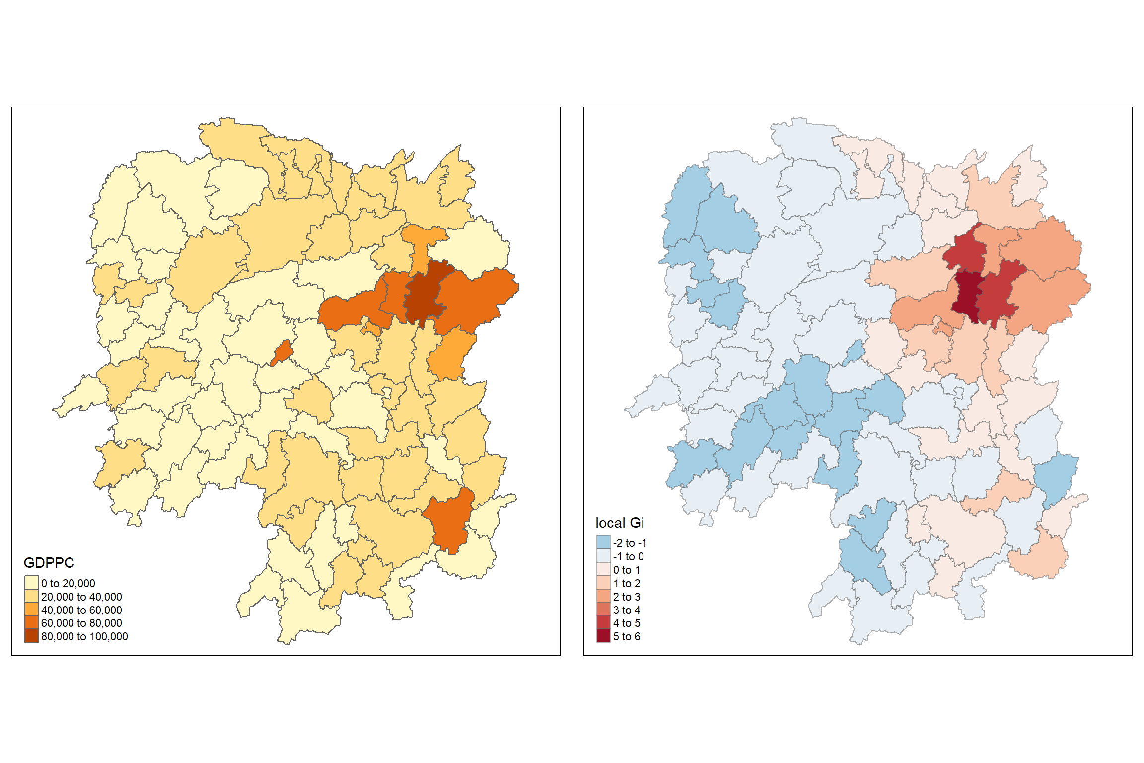
The Gi* map (Getis-Ord Gi* statistic) for the GDP per Capita of counties in Hunan, China, suggests spatial hotspots and cold spots of economic wealth. The map on the right indicates areas with high Gi* values (in red), revealing clusters of counties with significantly high GDP per Capita—these are the hotspots of economic activity. Conversely, the blue areas represent cold spots with low Gi* values, indicating clusters of counties with low GDP per Capita. Notably, the central to northeast region shows a strong concentration of wealth with a Gi* value between 5 to 6, indicating a very high degree of clustering of economic affluence. This pattern highlights the unequal distribution of economic wealth across the region, with certain areas being significantly more prosperous than others, which can inform targeted economic development and policy intervention strategies.
Now, we repeat the process using an adaptive distance weight matrix (knn_lw). This allows us to consider different distances for each location based on their neighbors, providing a more flexible approach.
The Gi values based on adaptive distance weights are joined to the original data frame. Again, we visualize these values on a choropleth map to observe patterns.
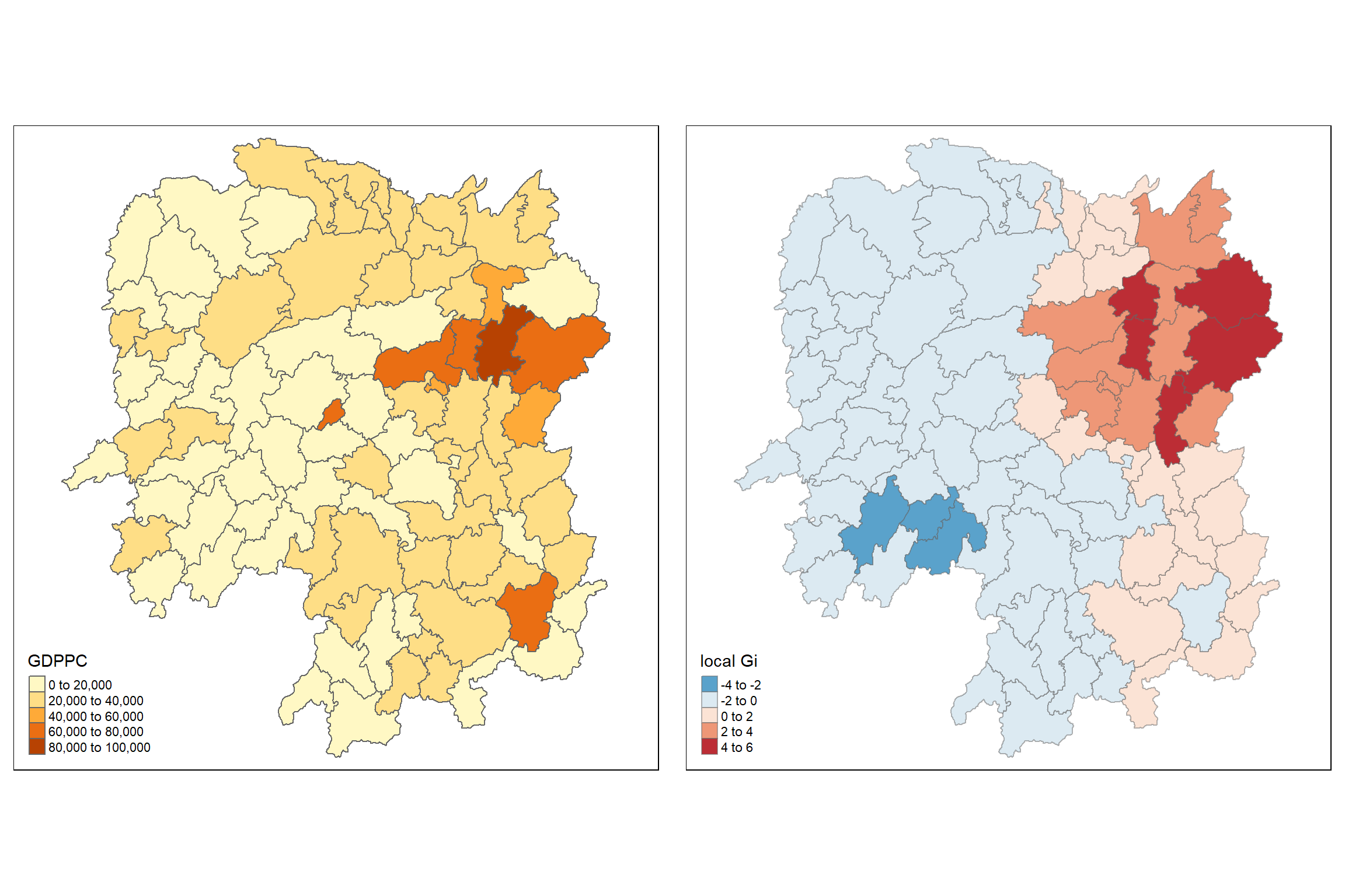
The Gi map with adaptive distance shows a clear delineation of economic clustering across the Hunan area. Compared to the previous fixed distance Gi map, the adaptive distance approach may provide a more nuanced view of spatial relationships, adjusting for varying densities of counties. This can highlight economic disparities more precisely, as the fixed distance may overemphasize or underrepresent clustering due to uniform application of distance across varied geographical spaces. The adaptive map might therefore offer a more accurate representation of spatial economic patterns, potentially revealing more localized clusters that are not as apparent with a fixed distance approach.